An Improvement to Calculation of Lighting Energy Requirement in the European Standard EN 15193:2007

Meng Tian; Yuehong Su

doi:10.15627/jd.2014.3

Article outline

3. Applicability of EN 15193 for wider locations

4. Improved correlation coefficients for better applicability of EN 15193

Figures and tables

Figures (18)

Tables (7)

Volume 1 Issue 1 pp. 16-28 • doi: 10.15627/jd.2014.3

An Improvement to Calculation of Lighting Energy Requirement in the European Standard EN 15193:2007

Meng Tian, Yuehong Su^*

Author affiliations

Institute of Sustainable Energy Technology, Department of Architecture and Built Environment, University of Nottingham, University Park, NG7 2RD, UK.

* Corresponding author. Tel.: +82 10 27477520; fax: +44 115 9513159
Meng.Tian@nottingham.ac.uk (M. Tian)
yuehong.su@nottingham.ac.uk (Y. Su)

History: Received 5 September 2014 | Revised 22 November 2014 | Accepted 15 November 2014 | Published online 1 Dec 2014

Citation: Meng Tian and Yuehong Su, An Improvement to Calculation of Lighting Energy Requirement in the European Standard EN 15193:2007, Journal of Daylighting 1 (2014) 16-28. http://dx.doi.org/10.15627/jd.2014.3

Figures and tables

Figure 1
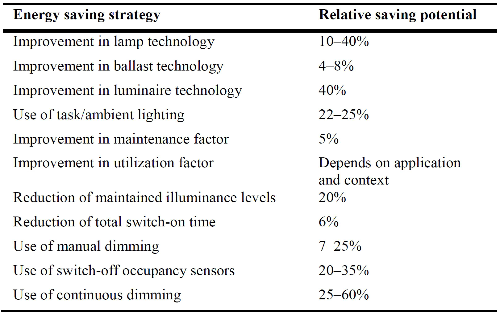Table 1
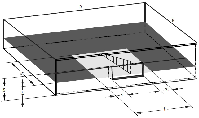Figure 2
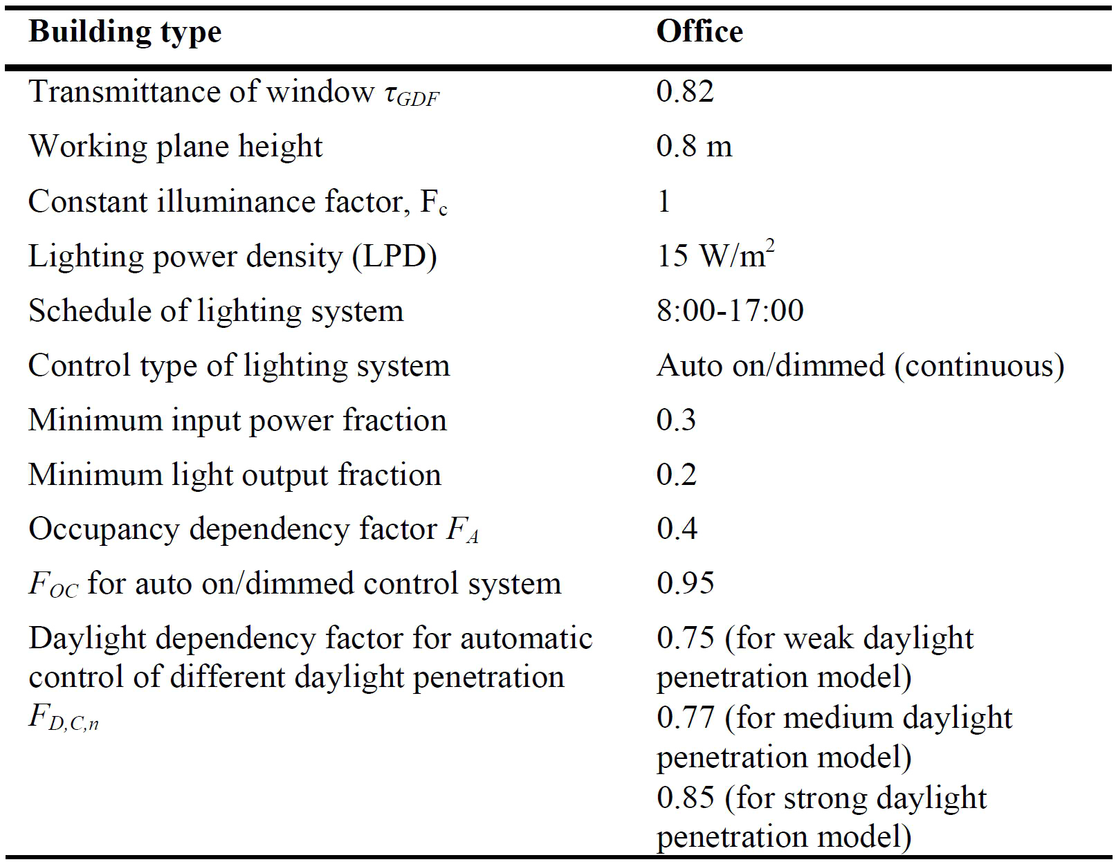Table 2
Figure 3
Table 3
Table 4
Figure 4
Figure 5
Figure 6
Figure 7
Figure 8
Table 5
Figure 9
Table 6
Figure 10
Table 7
Figure 11
Figure 12
Figure 13
Figure 14
Figure 15
Figure 16
Figure 17
Figure 18

Abstract

Daylighting has a recognized potential for electric energy savings when is used as a complement for artificial lighting. This study reviews the comprehensive calculation method for lighting energy requirement in non-residential buildings introduced by the European Standard EN 15193: 2007 and investigates its feasibility in China. The location of building influences the intensity and duration of daylight. In EN 15193 calculation method, the daylight supply factor, which represents the effect of daylighting on usage of artificial lighting, is the only factor related to location and calculated according to latitude, however the current method (EN15193: 2007) limits the latitude range from 38° to 60° north in Europe, for which the relationship between daylight supply factor and latitude is approximately linear. This study shows that a quadratic relationship needs to be used for a wider range of latitudes. The coefficients of the proposed quadratic relationship are determined for the classified daylight penetration and maintained illuminance level. Various control types are also considered. Prediction of energy requirement for lighting is obtained through building simulation tool EnergyPlus and the effects of some setting factors are discussed.

Keywords

Daylighting; Daylight supply factor; Daylight penetration; Illuminance level

Nomenclature

F_A	Absence factor
F_C	Constant illuminance factor
F_D	Daylight dependency factor
F_D,n	Daylight dependency factor in room or zone n
F_D,C,n	Daylight dependent electric lighting control factor in zone n
F_D,S,n	Daylight supply factor in zone n
F_o	Occupancy dependency factor
F_OC	Occupancy dependent lighting control system factor
MF	Maintenance factor
P_n	Total installed lighting power in the room or zone [W]
P_pc	Total installed parasitic power of the controls in the room or zone [W]
P_em	Total installed input charging power of the emergency lighting luminaires in the room or zone [W]
t_D	Daylight time usage [h]
t_N	Non-daylight time usage [h]
t_y	Standard year time [h] (8760h)
t_em	Emergency lighting charge time [h]
W	Total annual energy used for lighting [kWh⁄(year])
W_t	Total energy used for lighting [kWh]
W_L,t	Energy consumption used for illumination for the period t [kWh]
W_L	Annual lighting energy used [kWh⁄(year])
W_P	Annual parasitic energy used [kWh⁄(year])
W_P,t	Luminaire parasitic energy consumption for the period t [kWh]
γ_site	Latitude of building location [°]

1. Introduction

Lighting systems take a percentage of about 20–60 of the annual energy consumption in non-residential buildings, which is about one-third of the electricity budget [1,2]. Figure 1 shows energy consumption of two typical office buildings, one is naturally ventilated and the other is air-conditioned [3]. The proportions occupied by the lighting system are illustrated clearly.

Figure 1

Fig. 1. Energy use indices (EUIs) for typical examples of two office types [3].

There are two main aspects of energy saving for electric lighting, one is about installation of electric lighting and the other is in regards to daylight harvesting. The first one includes the improvements of technologies of the lamp itself and control systems. In respect to daylight harvesting, the effects of location, window characteristics, shading, building structure and reflectance of inner surfaces are taken into consideration. The overall lighting design combines the choice of lighting facilities and design of control system [4]. Lamps and fittings determine the major cost of energy use and an efficient control system provides a further energy saving. Table 1 gives several approaches to reducing the energy use of electric lighting. The relative saving potential of each strategy is demonstrated as well.

Table 1

Table 1. Energy saving strategies and relative energy saving potential [5].

The energy use of artificial lighting systems could be reduced efficiently by integrating daylighting and artificial lighting systems, which is regarded as one of the simplest ways to improve the energy efficiency of buildings [5,6]. The benefits of daylight are mainly embodied in two aspects which are visual comfort and psychological comfort. In respect of economy, the improvements of lighting is considered as the best investments in most non-residential buildings due to the large proportion of energy bill, which ranges from 30% to 70% of total energy budget [7]. In addition, daylighting is a great choice to prevent environmental pollution of CO₂ emissions and global warming to which artificial lighting systems are the major contributors.

There are two main types of daylighting controls given by IESNA [8], one is switching controls and the other is continuous dimming control. An appropriate integration of control and lighting systems could obtain effective energy saving results. Many studies have discussed the contributions of lighting control for energy saving in buildings. Ihm, Nemri and Krarti [9] conducted a research of energy saving potential of daylighting for a small office space in Boulder, USA. The results indicated that 60% annual energy saving could be achieved by using dimming control. Based on field measurements on daylighting in a fully air-conditioned daylit corridor in Hong Kong, Li and Lam [10] found the substantial energy savings of electric lighting. The annual saving was up to 70% by using dimming control systems and about 47.2 kWh/m approximately.

With the fast economic growth in China since 1990s, the total electricity consumption of China rose from 612.6–3658.7 TWh [11]. In 2008, the total electricity consumption of lighting accounted 12% of total electricity consumption in China [11]. In addition, about 10–20% lamps of the 15 billion produced lamps were sold in China according to the data of 2008 [12]. It can be seen that there is a high potential of energy saving with respect of lighting energy consumption in China nowadays. Saving energy in lighting has already been advocated by many European countries for many years, but it just caught more attention in China in recent years. Therefore, introducing the calculation methodology in respect of lighting energy from Europe is significant to China. The international cooperation will be enhanced as well.

European Standard EN 15193:2007 [13] establishes the calculation methodology for estimating the amount of energy consumption for lighting in buildings and gives a numeric indicator for lighting energy requirements for certification purpose. Three different approaches for lighting energy evaluation in non-residential buildings are introduced by EN 15193:2007 [13], which are quick method, comprehensive method and metering. The quick method is based on the numeric indicator to calculate the lighting energy consumption, which means all of the coefficients are using default values during the calculations. The comprehensive method is more accurate comparing with the quick method which is suitable for calculating any periods and any locations and without use of default values. Metering evaluates the lighting energy consumption from the practical records of the target building. Unfortunately, the standard is only devised for countries in Europe located within the range of 38° to 60°N latitude. A report published in [14] put forward some modification of the coefficients in EN 15193, such as daylight supply factor and building orientations. It also mentions the Tabular method with less accuracy and Simplified method with higher accuracy compared to the simulation results in calculating the lighting energy consumption in buildings. In [15], they investigated the accuracy of EN 15193 predictions of lighting energy consumption by using the software Radiance, and the results shows that the deviations change with the different user behaviors.

This paper focuses on the manual calculation method of EN 15193:2007, and investigates the feasibility of it in other cities beyond the limited region in or near Europe and the cities in China. Therefore the comprehensive method is more suitable and accurate for making comparisons. The calculation steps of comprehensive method will be introduced briefly in this paper. Then simulations are put forward using the software EnergyPlus to investigate the influence caused by daylighting on the energy requirement of electric lighting systems. Both of the results from manual calculation and simulation will be compared and discussion about deviations will be introduced. After the analysis, the feasibility of comprehensive method by EN 15193:2007 in other locations beyond the limited region in or near Europe and China will be evaluated. New correlations of building location and lighting energy will be determined by data regression and be classified for various daylight penetration and maintained illuminance levels. Other factors that have not been referred to the comprehensive method, such as minimum settings, will also be discussed to improve the correlation of building location and lighting energy. The results presented by this paper may be useful to the future amendment of the current EN 15193:2007.

The remainder of the paper is organized in the following manner. Section 2 describes the comprehensive method of the European Standard EN 15193: 2007 and Energyplus simulation as an approach to investigate this standard for potential improvement. Applicability of this European standard for China and other locations with a larger range of latitudes is discussed in Section 3 by comparing the EN15193 calculation and Energyplus simulation, and the sensitivity of this comparison is also discussed. This therefore leads to the suggestion of an improved correlation between daylight supply factor and latitude, as presented in Section 4. A further discussion about the contribution of this study and other potential improvements to this European standard is given in Section 5 while Section 6 summaries this study.

2. Methodology

The comprehensive calculation method for lighting energy requirement in the European Standard EN 15193: 2007 [13] will be introduced briefly and the approach to improving this method will be described.

2.1. Comprehensive method of EN 15193: 2007

2.1.1. Estimation of lighting energy requirements

The total energy required for a period in a room is calculated by

\[ W_t = W_{L,t} + W_{P,t} ~ ~ ~ ~ [kWh] \]

where W_L,t is the lighting energy required to fulfil the illumination function in a room for dimming-control period and full-power period:

\[ W_{L,t} = \sum\frac{(P_n \times F_c)\times\left ](t_D \times F_o \times F_{D,n})+(t_N \times F_o)\right ]}{1000} ~ ~ ~ ~ [kWh] \]

where W_P,t is the parasitic energy required to provide charging energy for emergency lighting and for standby energy for lighting controls in the building:

\[ W_{P,t} = \sum \frac { \lbrace P_{pc} \times \left [(t_y - (t_D + t_N) \right ] \rbrace + (P_{em} \times t_{em})}{1000} ~ ~ ~ ~ [kWh] \]

where T_D and T_N are the default values for annual operating hours which depends on the building types. Total annual energy use for lighting is the sum of W_L,T and W_P,T over the period of one year:

\[ W = \sum W_{L,t} + \sum W_{P,t} = W_L + W_P ~ ~ ~ ~ \left [\frac {kWh}{year}\right ] \]

If the real consumption data of parasitic energy for the building is available, it should be used. The default energy consumption of parasitic energy that consists of 1 kWh/(m² × year) for emergency lighting and 5 kWh/(m² × year) for the automatic lighting controls if used, which means the total consumption for parasitic energy is 6 kWh/(m² × year) is applied only if the real values are missing.

2.1.2. Daylight dependency factor F_D

Daylight dependency factor is determined by:

\[ F_{D,n} = 1 - \left (F_{D,S,n} \times F_{D,C,n}\right ) \]

where F_D,C,n is daylight dependent artificial lighting control factor, which depends on the type of control system of artificial lighting and daylight penetration, the values are illustrated in Table 2. F_D,S,n is daylight supply factor:

Table 2

Table 2. Specification of models [13].

\[ F_{D,S,n} = \alpha + b ~ \gamma_{site} \]

where γ_site is the latitude ranging from 38° north to 60° north; a and b are coefficients determined by the maintained illuminance level and daylight penetration.

2.1.3 Occupancy dependency factor F_o

\[ F_o = 1 - \left [ \frac {(1 - F_{OC}) \times F_A}{0.2} \right ] ~ when ~ 0 \leq F_A < 0.2 \]

\[ F_o = F_{OC} + 0.2 - F_A ~ when ~ 0.2 \leq F_A \leq 0.9 \]

\[ F_o = \left [ 7 - (10 \times F_{OC}) \right ] \times (F_A - 1) ~ when ~ 0.9 \leq F_A \leq 1.0 \]

where F_A is the factor depends on the building type and FOC is the factor depends on the type of control systems.

2.1.4. Constant illuminance factor F_C

Constant illuminance factor is the ratio of the average input power over a given time to the initial installed input power to the luminaire, i.e.

\[ F_C = \frac {1 + MF}{2} \]

where MF is the maintenance factor for the scheme. In this study, MF = 1 is used.

2.1.5. Daylight factor

The impact of the fenestration and sun-protection system could be judged by daylight factor DC. The strong daylight penetration requires a daylight factor DC >= 6%. When 6% > DC >= 4%, the daylight penetration is medium and the weak daylight penetration is 4% > DC >= 2%. There is negligible daylight penetration when DC < 2%. The daylight factor for carcass façade opening is calculated by

\[ D_C = (4.13 + 20.0 \times I_T - 1.36 \times I_{De}) ~ I_O ~ (\%) \]

where D_C is the daylight factor. IT is the transparency index:

\[ I_T = \frac {A_C}{A_D} \]

where A_C is the area of the façade opening [m2], and AD is the total area of daylight zone benefiting from natural lighting [m].

Figure 2

Fig. 2. Daylight zone for a room with small façade opening and larger room depth [13].

The daylight zone is an area in a room receiving daylight. In Fig. 2, we show a daylight zone in a room with small façade opening and larger room depth as an example. The maximum depth of the daylight zone [m], a_D,max, given by:

\[ A_{D,max} = 2.5 \times (h_{Li}-h_{Ta}) \]

where h_Li is height of the lintel above floor [m] and h_Ta is height of the working plane above floor [m]. The total area of the daylight zone is calculated by:

\[ A_{D} = a_D \times b_D \]

where a_D is the depth of daylight zone [m]. If the actual depth of a zone is smaller than the calculated a_D,max of the daylight zone, the actual depth of the zone can be taken as the value of aD. If the actual depth of a zone is less than 1.25 times a_D,max, the calculated a_D,max can be used for a_D. I_De is the depth index of the daylight zone:

\[ I_{De} = \frac {a_D} {h_{Li} - h_{Ta}} \]

1: b_D is the width of daylight zone [m]; 2: a_D,max/4; 3: a_D,max/4; 4: h_Ta height of task area (the working plane) above floor [m]; 5: h_Li height of lintel above floor [m]; 6: aD,max maximum depth of daylight zone [m]; 7: b_R width of room [m]; 8 a_R depth of room [m] (Fig. 2).

I_O is the correction factor for obstruction and is calculated by the correction factor for glazed double facades according to the model in this paper, i.e.

\[ I_O = \tau_{GDF}K_{GDF1}K_{GDF2}K_{GDF3} \]

where τ_GDF is the visible transmittance of glazed double façade; k_GDF1 is the factor account for frames of glazed double façade (0.8 in general); k_GDF2 is the factor accounting for dirt of glazed double façade (1 in general); k_GDF3 is the factor accounting for not normal light incidence on façade (0.85 in general).

2.2 Model description

According to the manual calculation method, three models with weak, medium and strong daylight penetration were created to perform different daylight conditions. The geometry of each model is demonstrated in Fig. 3. All the models were assumed for offices with corresponding working schedule. In order to better verify models, three levels of maintained illuminance are set as references, which are 300 lux, 500 lux and 750 lux, same as the illuminance levels applied in EN 15193:2007 [13]. Two sensors are located at the height of working plane symmetrically, and each controls half of the room lamps. The assumption of lighting power density (LPD) is 15W/m² which is the benchmark value of office lighting power density provided in EN15193, and it is also referred in CIBSE Guide A [16] as a common value. The control system of lighting is assumed to be auto on/dimmed. The minimum input power fraction is the lowest power the lighting system can dim down to under the continuous dimming control system. The minimum output fraction is the lowest light output the lighting system can dim down to and it occurs when the system produces at minimum input power. The 0.2 light output fraction and 0.3 input power fraction are the default values in EnergyPlus which are the common properties of continuous dimming control system nowadays. The windows of models are double glazed. More details are demonstrated in Fig. 3.

Figure 3

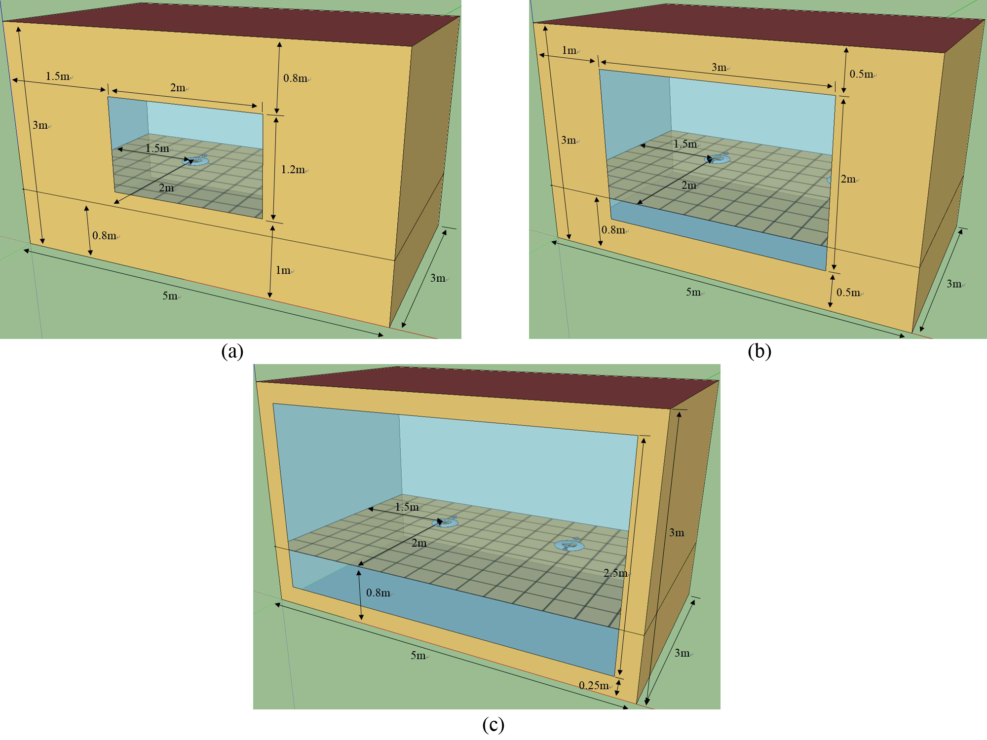
Geometry of simulation models. (a) Model A: weak daylight penetration and DC = 2.59%. (b) Model B: Medium daylight penetration and DC = 4.93%. (c) Model C: strong daylight penetration and DC = 8.54%.

Fig. 3. Geometry of simulation models. (a) Model A: weak daylight penetration and DC = 2.59%. (b) Model B: Medium daylight penetration and DC = 4.93%. (c) Model C: strong daylight penetration and DC = 8.54%.

2.3 Methodology

According to the comprehensive method introduced in Section 2.1, it could be seen that the only item relating to location is daylight supply factor F_D,S,n determined by Eq. (6). Therefore, the results used to compare with simulation results is the lighting energy required to fulfill the illumination function W_L,t. The parasitic energy need not to be taken into consideration. To estimate the coefficients a and b in Eq. (6) for other locations, which would be different from those in Table 3, the energy consumption was first predicted by using the simulation tool, EnergyPlus, which is capable of modeling the whole building energy performance including thermal performance and HVAC systems. In particular, the results of energy consumption of the lighting system were used to give W_L,t and then determine F_D,n from Eq. (2).

Table 3

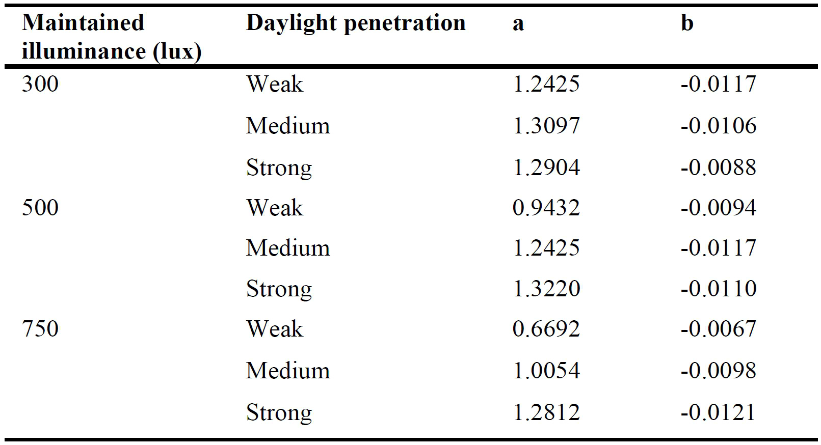
Table 3. Coefficients a and b of Eq. (6) for various maintained illuminance and daylight penetration in EN 15193:2007.

In addition, because the manual calculation based on EN 15193 restricts the cities positions to the location within the latitudes ranging from 38° to 60° N in Europe, the applicability of manual calculation method for the cities beyond limited latitude range in or near Europe and China will be therefore explored by comparing the results from manual calculation and simulation. Finally, the amendments of Eq. (6) will be put forward based on the obtained F_D,n from Energyplus simulation.

3. Applicability of EN 15193 for wider locations

In this study, 14 Cities in or near Europe and 24 cities in China with different latitudes are chosen to explore the applicability of the manual calculation method for the cities beyond the region given in EN 15193:2007. Their names and latitudes are demonstrated in Table 4. The following Sections 3.1 and 3.2 illustrate the results for these cities and the discussion of deviations is put forward in Section 3.3.

Table 4

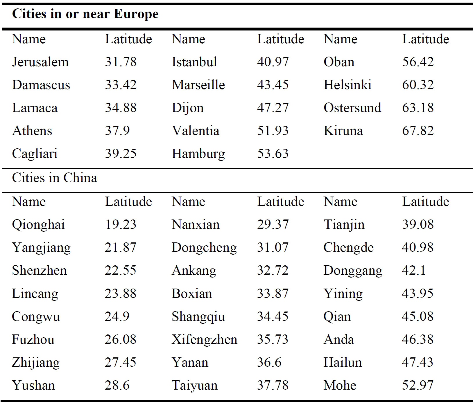
Table 4. Selected cities and latitudes.

3.1 Applicability for cities in or near Europe

To validate the calculation method of EN 15193:2007, Fig. 4 shows the results for those cities in or near Europe. The deviation in lighting energy requirement between the Energyplus simulation and EN 15193 is defined by:

\[ Deviations = \frac {Simulation ~ results - EN ~ 15193 ~ results}{EN ~ 15193 ~ results} \]

Figures 4(a), (b) and (c) are for weak, medium and strong daylight penetration, respectively. Each of them includes three different illuminance set point (maintained illuminance), which are 300 lux, 500 lux and 750 lux. According to the labels and the orange vertical marked lines of each figure, it is easy to see the cities located within or beyond the region from 38° to 60° N in or near Europe. The dispersion of points illustrates tendencies of the relationship between deviations and latitudes. In general, the weaker daylight penetration results in the smaller deviations. The deviation is larger for the cities with the latitude smaller than 38^oC.

Figure 4

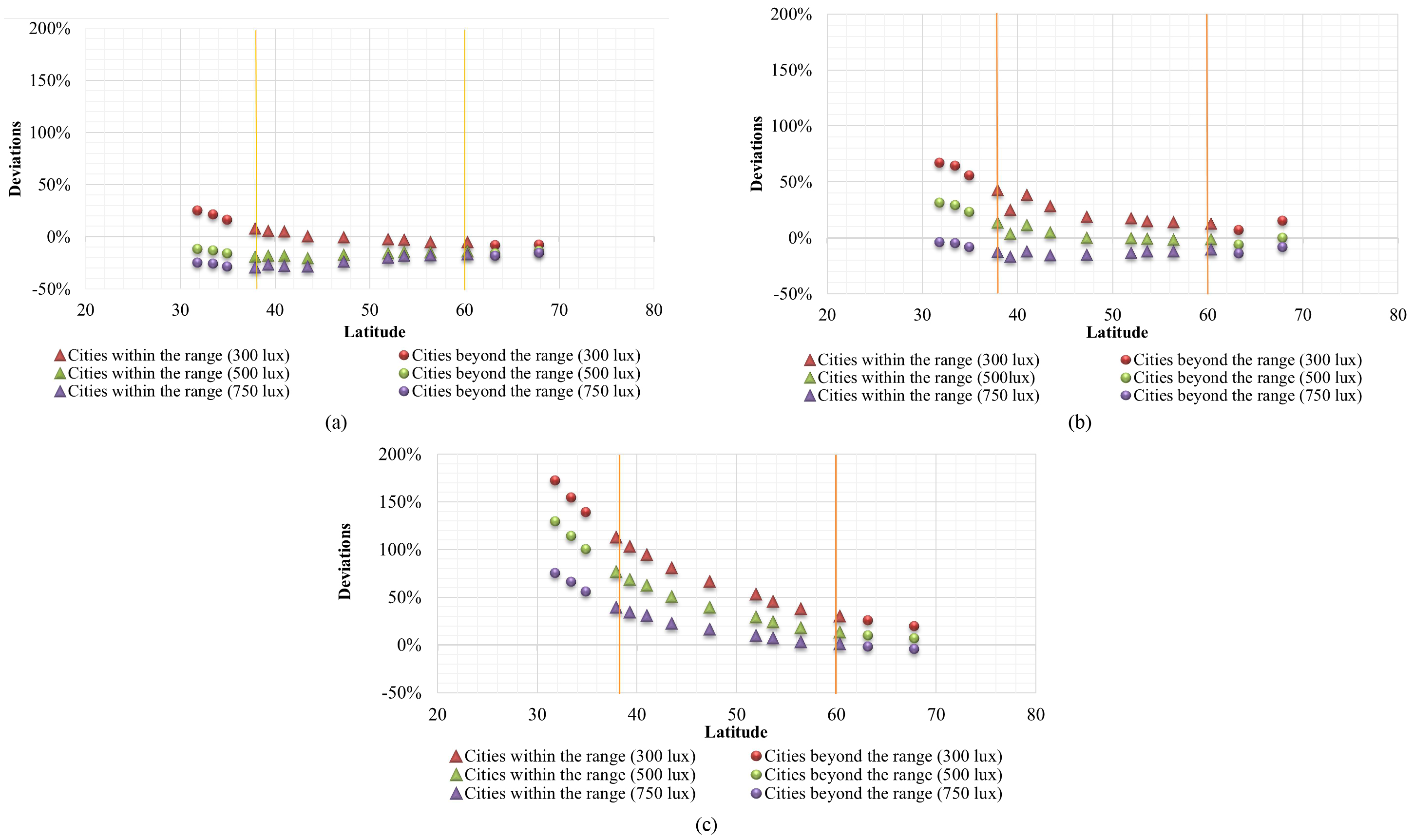
Fig. 4. Deviations of lighting energy requirement for those cities in or near Europe for (a) weak, (b) medium, and (c) strong daylight penetration.

3.2 Applicability for cities in China

The applicability of EN 15193 for China is a focus of this study. As shown in Fig. 5, most of the cities in China are located in the lower latitude comparing with those cities in or near Europe. Similar to the results in previous section, the cities with lower latitude present a larger deviation, regardless of different daylight penetration and maintained illuminance.

Figure 5

Deviations of lighting energy requirement for those cities in China and in or near Europe for (a) weak, (b) medium, and (c) strong daylight penetration.

Fig. 5. (a) Deviations of lighting energy requirement for those cities in China and in or near Europe for (a) weak, (b) medium, and (c) strong daylight penetration.

3.3 Discussions of applicability

Deviation can be seen from the comparison of simulation and EN 15193 results. Because of the limitation on latitude range in EN 15193, the deviation becomes large for the locations out of the range of latitudes. In this section, the results are discussed in different aspects in order to explore the factors that affect the deviations. In addition, the relationship between them will be investigated in order to put forward potential improvements to EN 15193, as given in the next section.

3.3.1 Effect of illuminance level set point

The set point of illuminance influences the results of lighting energy requirement and the deviations between simulation and EN 15193 results. Figures 4 and 5 demonstrate the deviations in lighting energy requirement for different maintained illuminance levels of 300, 500, and 750 lux, respectively. It could be seen that thier tendencies of the deviations are the same; while the larger maintained illuminance level corresponds to the smaller differences under the same conditions of latitude and daylight penetration. The reason for this may be because of different fluctuation of solar radiation in different cities. The lighting energy requirements of spaces with higher illuminance set points are less sensitive to the local weather conditions; as it is considered in the standard-based equations, it would be retained when the equations are improved.

3.3.2 Effect of daylight penetration

The effect of daylight penetration can be seen from Fig. 4 for a given maintained illuminance level such as 500 lux. The tendencies are quite similar between three illuminance levels, but the deviations go higher from weak, medium to strong daylight penetration, particularly within the range of lower latitudes.

3.3.3 Effect of sensor position

The sensor position will influence the detection of the amount of daylight. The deeper of the sensor is located, the less daylight can be detected. In order to investigate the effects of sensor position, the sensors are put in four different positions, which are 1.5 m, 2 m, 2.5 m, and 3 m away from the window. The results in Fig. 6 show that the effects on deviations by the sensor positions are almost independent of latitude, so this factor would not be discussed for the intended improvement to the standard EN 15193. The generally recommended sensor position of 2 m would be used in the following discussions.

Figure 6

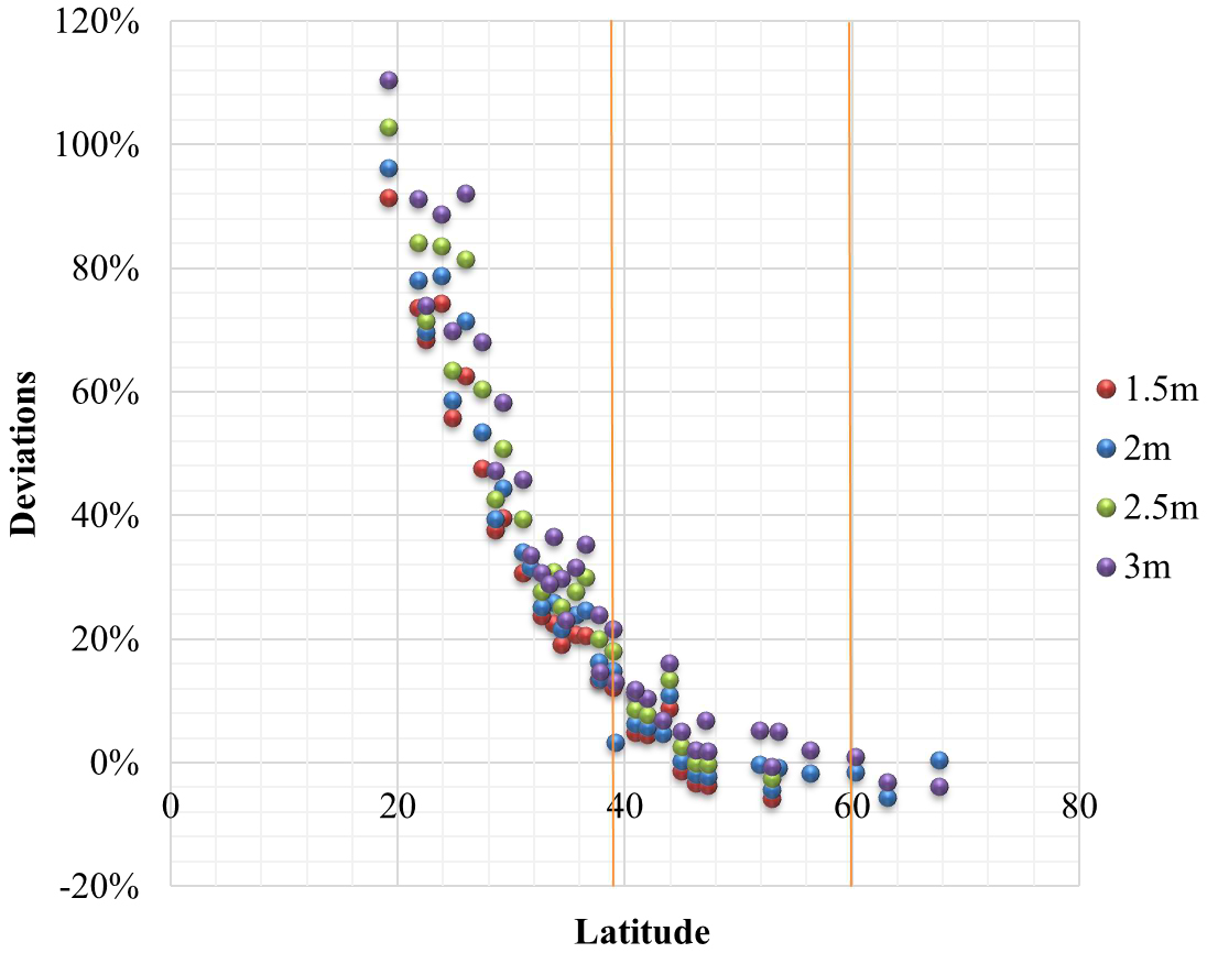
Deviations of lighting energy requirement for different sensor positions for the condition of medium daylight penetration and 500 lux maintained illuminance.

Fig. 6. Deviations of lighting energy requirement for different sensor positions for the condition of medium daylight penetration and 500 lux maintained illuminance.

3.3.4 Effect of model geometry

This section is to investigate the effects of different model geometry within the same range of daylight penetration. Seven cities (Table 5) in or near Europe were chosen for comparison. The daylight penetration of both models (Figs. 7 and 8) are weak, i.e., 2% < DC < 5%.

Table 5

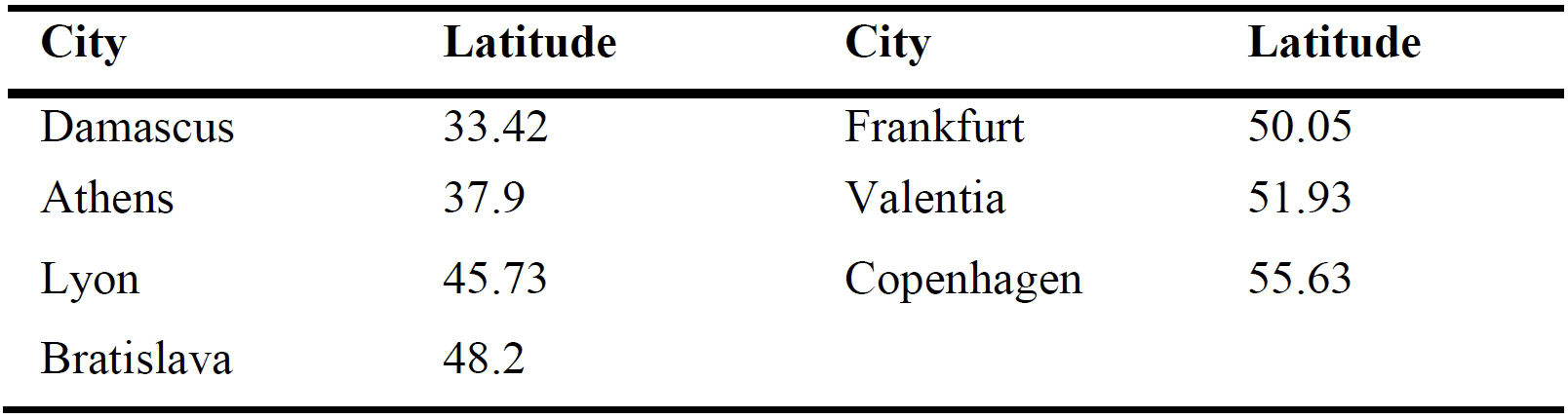
Table 5. Selected cities and latitudes.

Figure 7

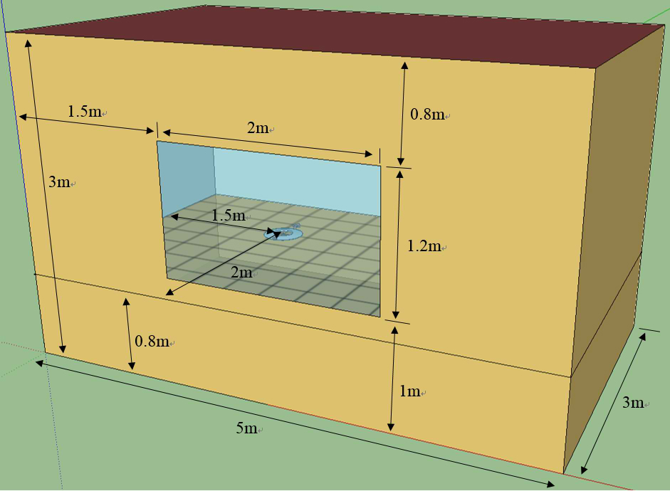
Fig. 7. Original model with weak daylight penetration (Daylight factor 2.59%).

Figure 8

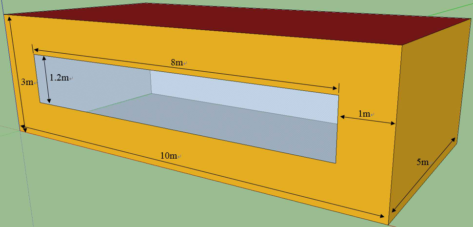
Fig. 8. Amended model with weak daylight penetration (Daylight factor 3.6%).

The results are compared in Fig. 9. For the models with weak daylight penetration, it is clear that the deviations are almost the same regardless of the model performance. Hence, this factor would not be considered for the intended improvement.

Figure 9

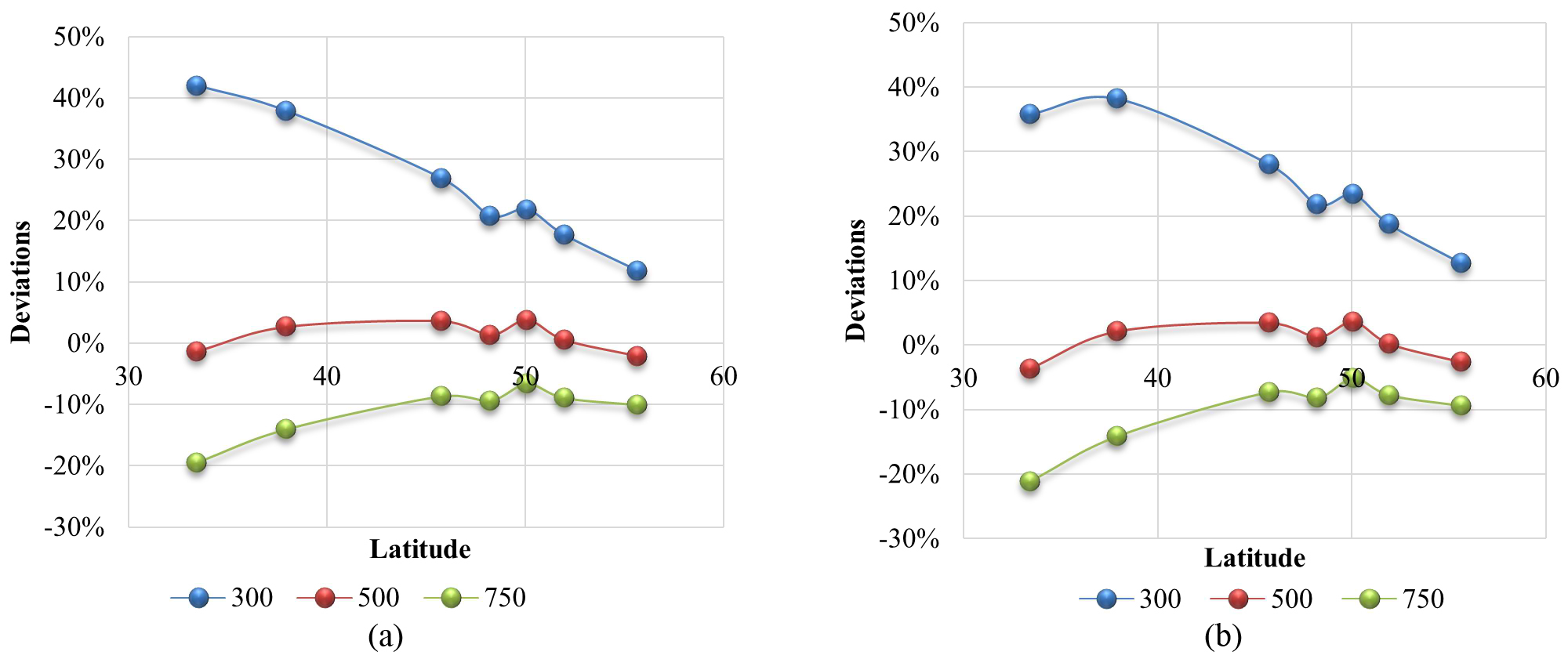
Comparison of deviations in lighting energy requirement for different models with weak daylight penetration for (a) original model and (b) amended model.

Fig. 9. Comparison of deviations in lighting energy requirement for different models with weak daylight penetration for (a) original model and (b) amended model.

4. Improved correlation coefficients for better applicability of EN 15193

According to the discussions, seven factors are likely to influence the deviations in lighting energy requirement between Energyplus simulation and manual calculation results by EN 15193. They are summarized in Table 6 in which the effects and treatment are demonstrated as well. The comprehensive calculation method of European Standard EN 15193 would be improved for the selected influence factors. The coefficients in those equations will be discussed separately based on the different maintained illuminance levels and daylight penetration. In addition, the relationship between lighting energy requirement and minimum settings of high frequency dimming control will be put forward. Other factors would not be discussed because some of them have no obvious effect.

Table 6

Table 6. Summary of influence factor.

4.1 New correlation of daylight supply factor

4.1.1 Determination of coefficients

In EN 15193 comprehensive calculation method as described in Section 2, Eq. (6) is the only equation that is affected by the latitude of a location. Therefore, to improve the applicability of EN 15193, the relationship between the daylight supply factor and latitude is focused. In Fig. 10, we show such relationship for weak, medium and strong daylight penetration models with 500 lux maintained illuminance. The other two models with other illuminance set points have the similar relationships compared to this.

Figure 10

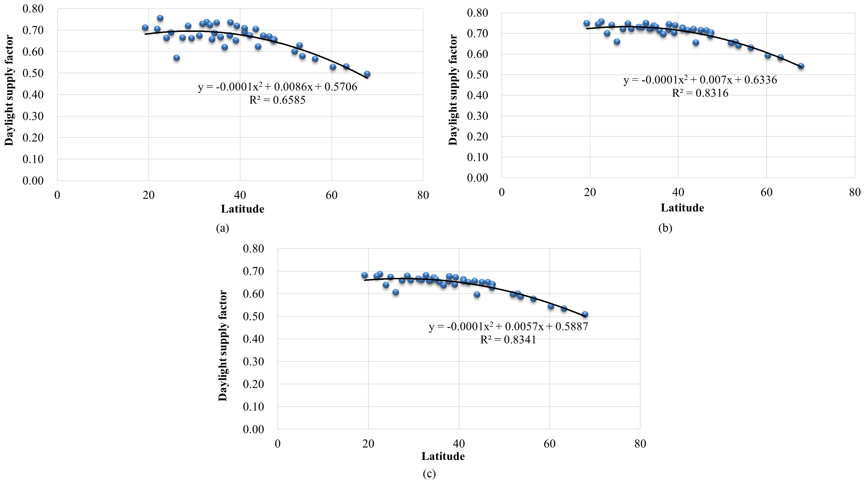
Relationship between daylight supply factor and latitude for different daylight penetration with 500 lux maintained illuminance for (a) weak, (b) medium, and (c) strong daylight penetration model.

Fig. 10. Relationship between daylight supply factor and latitude for different daylight penetration with 500 lux maintained illuminance for (a) weak, (b) medium, and (c) strong daylight penetration model.

The original Eq. (6) presents the relationship as linear function. However, according to Fig. 10, the dispersion of points indicates that the relationship of daylight supply factor and latitude have quadratic function for larger range of latitudes, i.e.

\[ F_{D,S} = a{\gamma_{site}}^2 + b\gamma_{site} + C \]

where F_D,S is daylight supply factor, γ_site is latitude, and a, b and c are constants.

The values of coefficients a, b and c are shown in Table 7 which are classified according to the different daylight penetration and maintained illuminance. R² is the coefficient of determination, and is generally lower for larger maintained illuminance and weaker daylight penetration.

Table 7

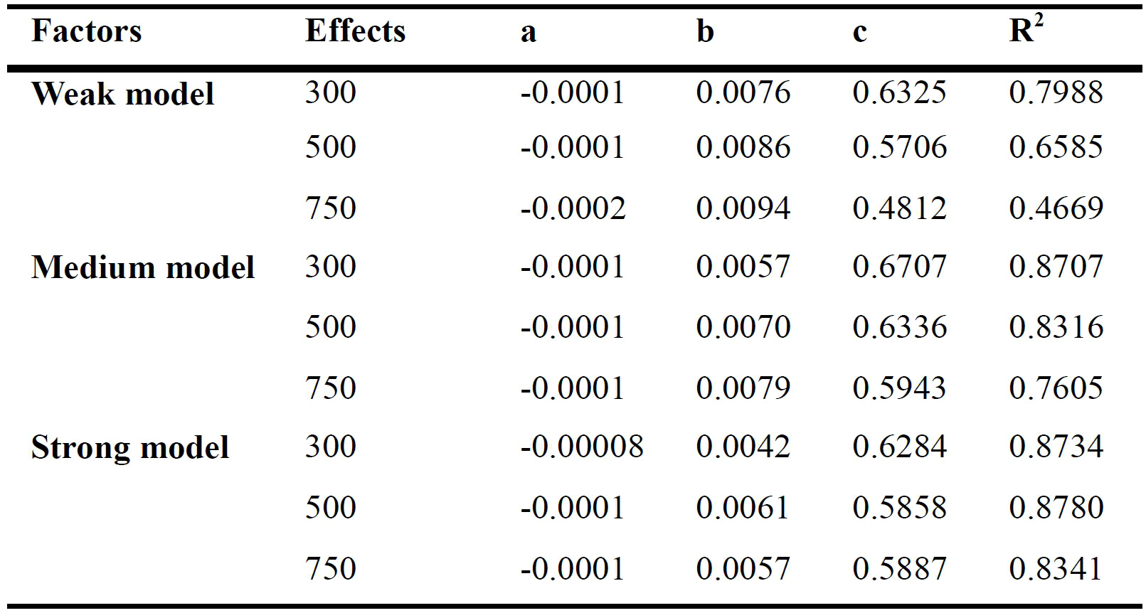
Coefficients for determining the daylight supply factor FD,S for vertical facades for various daylight penetration and maintained illuminance Em.

Table 7. Coefficients for determining the daylight supply factor F_D,S for vertical facades for various daylight penetration and maintained illuminance E_m.

4.1.2 Comparison with original correlation

In order to validate the new correlation, the deviations between Energyplus simulation and EN 15193 calculation by the improved correlation are compared with the original one, i.e., Eq. (6). The medium daylight penetration model with 500 lux maintained illuminance is shown in Fig. 11 as an example. It could be seen that the new correlation suits the cities located within the range of 18° to 70°N latitudes. The deviations between Energyplus simulation and EN 15193 calculation results for the original correlation goes as large as 100%, whereas the deviations by the improved correlation are lower than 20%. On the other hand, for the cities located in latitude from 50° to 70°N, the original linear correlation looks more suitable.

Figure 11

Layout of the SOEs of the Fresnel-based concentrators. All these concentrators have the same the same acceptance angle (α = ± 1 deg).

Fig. 11. Comparison of the original and improved correlations (medium daylight penetration with 500 lux maintained illuminance).

4.1.3 Validation analysis

Equation (18) as an improved correlation can be used to replace Eq. (6) for larger range of latitudes to extend applicability of European Standard EN 15193, while other equations are retained. Figure 12 demonstrates the validation results for the improved correlation. It can be seen that all of the deviations between the simulation and improved EN 15193 calculation results are decreased to ±25%. The larger deviations occur in the weak daylight penetration model because of the smaller coefficient of determination (R²). The reason for this is similar to that introduced in Section 3.3.1. The interior of the weak daylight penetration model receives less daylight compared to medium and strong model. Hence the maintained illuminance level is more difficult to achieve. Due to the fluctuation of solar irradiation under different weather conditions, the points of values for the weak daylight penetration model are more dispersed and with larger differences, which also result in the smaller value of R². However, the range of deviations could be accepted in the practical cases. The improved equation suits the strong daylight penetration model very well due to the higher value of R². The deviations are all close to 0%. In general, the improved correlations could be applied in cities within the range of 18° to 70°N latitudes.

Figure 12

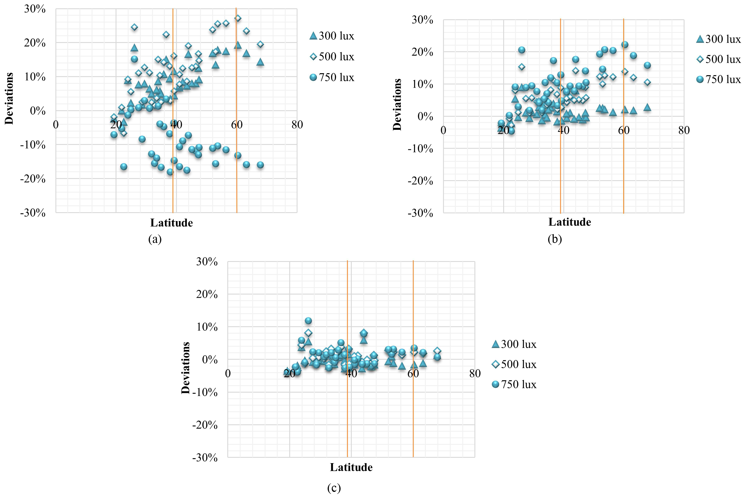
Deviations in lighting energy requirement between EnergyPlus simulation and improved EN 15193 (a) weak, (b) medium, and (c) strong daylight penetration model.

Fig. 12. Deviations in lighting energy requirement between EnergyPlus simulation and improved EN 15193 (a) weak, (b) medium, and (c) strong daylight penetration model.

4.2 Sensitive analysis

With the elimination of possible influence factors, three classified factors, which are daylight penetration, maintained illuminance and minimum settings, are discussed in this section in order to investigate their effects on the improved correlations.

4.2.1 Effect of maintained illuminance

Similar to Section 3.3.1, the influence of illuminance set points still exist. However, the offsets decrease significantly from 100% for the original correlation to 5–10% for the improved correlation, as shown in Fig. 12. The reason for this should be the different values of coefficient of determination (R²). For the weak daylight penetration model which has the lower value of R², the offset is about 10%. For the strong daylight penetration model, the higher value of R² result in the smaller offset which is only 2%. In general, the deviation caused by the maintained illuminance could be acceptable.

4.2.2 Effect of daylight penetration

For the original correlation, the effects of daylight penetration on deviations from Energyplus simulation results are as large as 400%, as in Section 3.3.2. In Fig. 13, we show the deviations for the improved correlation. The results of manual calculation are much closer to the simulation results. However, there is also about 5–10 10% offset due to the different daylight penetration. In practical cases, the range of differences would be acceptable.

Figure 13

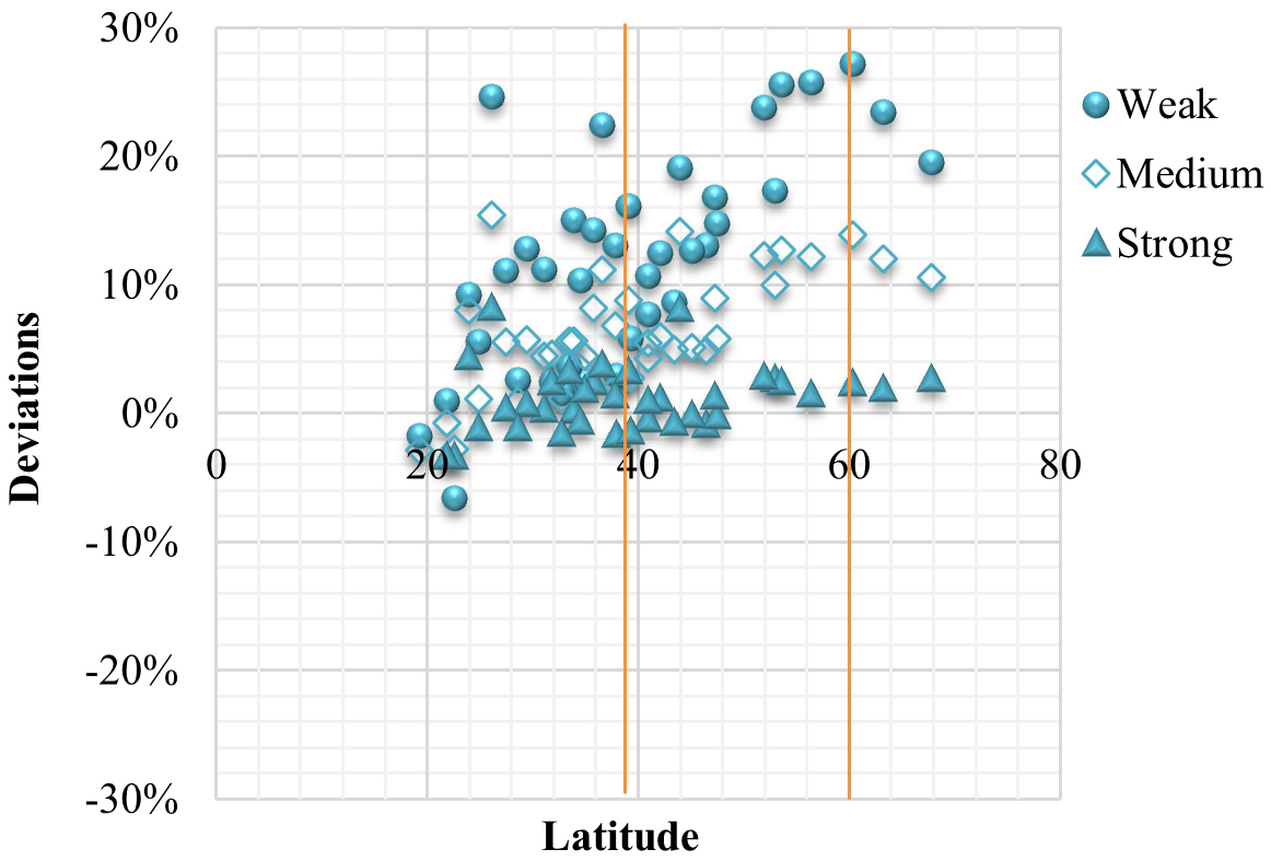
Deviations of lighting energy requirement between the simulation and improved EN 15193 for different daylight penetration model with 500 lux maintained illuminance.

Fig. 13. Deviations of lighting energy requirement between the simulation and improved EN 15193 for different daylight penetration model with 500 lux maintained illuminance.

4.2.3 Effect of minimum settings for dimming controls

The lighting control system assumed in this paper is high frequency dimming control, which relates to the sequential reduction of electrical lighting energy consumption due to daylighting. The ideal relationship between power input and light output of lighting is demonstrated in Fig. 14. The power input is almost by a linear function of the light output while the actual relationship depends on the type of dimming ballasts [17]. The power input and light output ratios are 0.3 and 0.2, respectively, for the reference case in Section 3.2.

Figure 14

Fig. 14. Correlation between light output ratio and power input ratio for an ideal high frequency dimming lighting control [18].

Figure 15 shows the effects of minimum settings on the deviation by the improved correlation from the simulation for the medium daylight penetration model with 500 lux maintained illuminance. Three combinations of minimum settings, (0.08,0.2), (0.2, 0.3) and (0.3, 0.4), were compared. Figure 16 shows the relationship between daylight supply factor and latitude for different combinations of minimum settings, which shows that there are about 0.15 offset of daylight supply factor for 0.1 power input interval. In order to decrease the deviations, the relationship between minimum settings, latitude and daylight supply factor is discussed as follows.

Figure 15

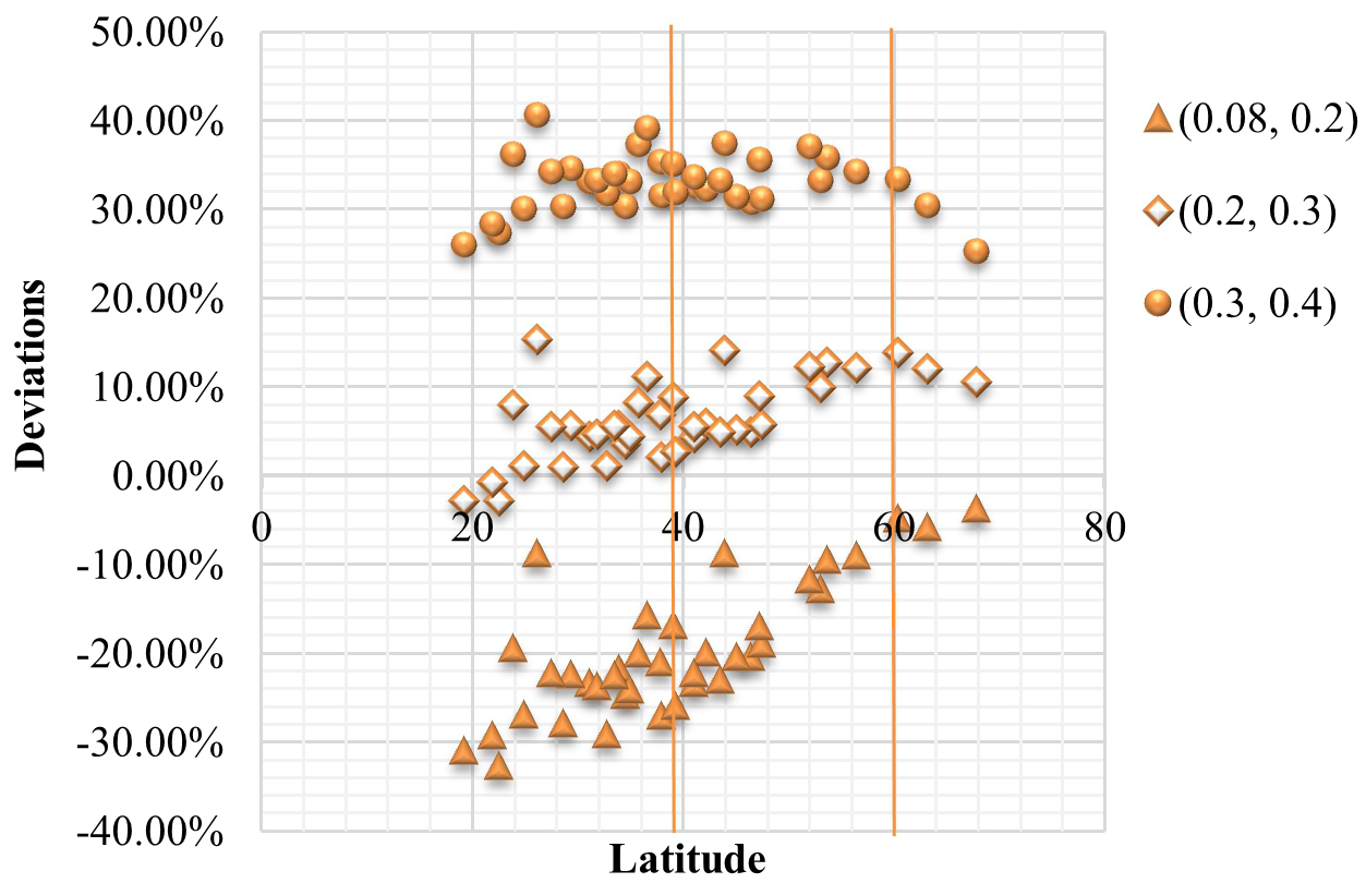
Effects on deviations by the improved correlation for various combinations of minimum settings for the medium daylight penetration model with 500 lux maintained illuminance.

Fig. 15. Effects on deviations by the improved correlation for various combinations of minimum settings for the medium daylight penetration model with 500 lux maintained illuminance.

Figure 16

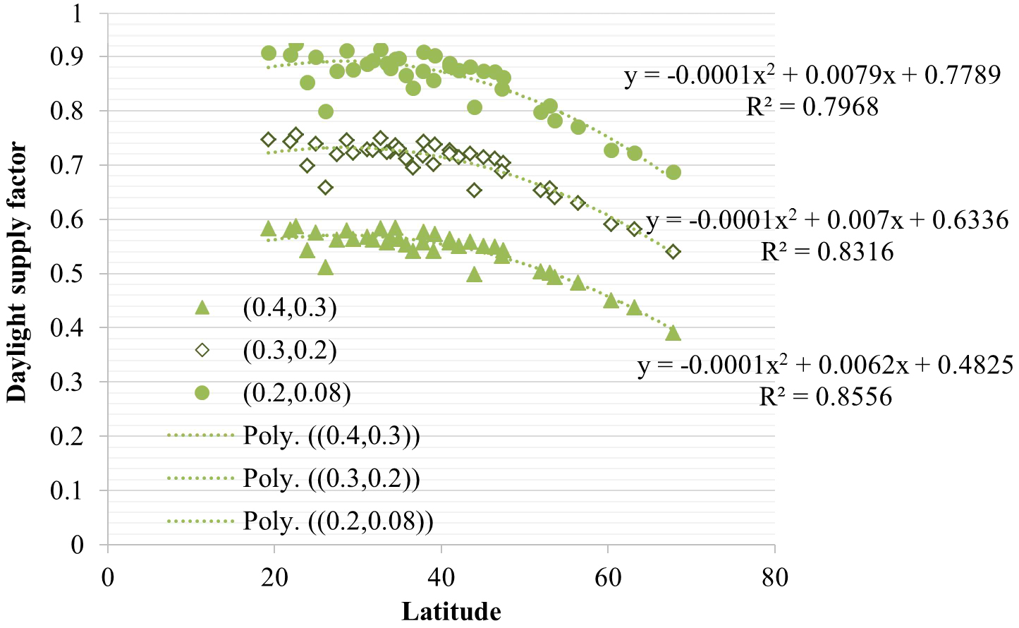
Relationship of daylight supply factor and latitude for various combinations of minimum settings for medium daylight penetration model with 500 lux maintained illuminance.

Fig. 16. Relationship of daylight supply factor and latitude for various combinations of minimum settings for medium daylight penetration model with 500 lux maintained illuminance.

Because the relationship of minimum light output and power input is almost linear for most ballasts, the improvement of the relationship between power input and coefficients of the correlation can be put forward. Figure 17 shows that the relationships between the power input ratio and both the coefficients b and c are linear, which could be written as Y=AX+B, where X is power input ratio and Y is coefficients b or c. The values of A and B are obtained from Fig. 17. These values are suitable for medium daylight penetration model with 500 lux maintained illuminance.

Figure 17

$Relationship of power input fraction and coefficients b and c for medium daylight penetration model with 500 lux maintained illuminance for coefficients (a) b and (b) c.$

Fig. 17. Relationship of power input fraction and coefficients b and c for medium daylight penetration model with 500 lux maintained illuminance for coefficients (a) b and (b) c.

In order to validate the correlation between the power input ratio and the coefficients a and b, the 0.4 power input and 0.3 light output ratios used as an example. The calculations are exemplified as below:

For coefficient b: b = – 0.0085 x 0.4 + 0.0096 = 0.0062

For coefficient c: c = – 1.482 x 0.4 + 1.0763 = 0.4835

Hence, the daylight supply factor for lighting system with 0.4 power input and 0.3 light output ratios is:

F_D,S = – 0.0001γ_site² + 0.0062 γ_site + 0.4835

The deviations in lighting energy requirement between simulation and improved EN 15193 results are shown in Fig. 18. The square points demonstrate the improved correlation and the circular ones demonstrate the original one. It can be seen that the improved correlation considering the minimum power input ratio is closer to the simulation results, with the deviation smaller than 10%. The coefficients given before are only suitable for the medium daylight penetration model with 500 lux maintained illuminance. For other conditions, the same analyzing process could be repeated and then obtain more accurate results. In addition, because of the limitation of the control system, this correlation is suitable for the ideal high frequency dimming control with the minimum power input ratio range of 0.2–0.4.

Figure 18

Fig. 18. Effects on deviations by the improved correlation for various combinations of minimum settings for the medium daylight penetration model with 500 lux maintained illuminance.

5. Discussions

This paper focuses on the validation of comprehensive calculation method devised by European Standard EN 15193:2007 for lighting energy requirement, in order to study its applicability for wider regions. This standard is limited to the cities located in or near Europe with the latitude ranging from 38° to 60° N. This paper has therefore investigated the applicability of this standard for the cities located within the latitudes ranging from 18° to 70°N in or near Europe and China. The initial results show that the models with weaker daylight penetration have smaller deviations between Energyplus simulation and EN 15193 calculation. This paper analyzed the reasons for deviation due to several factors such as illuminance level set point, daylight penetration, sensor position, model geometry, latitude, minimum dimming settings and solar irradiation. The locations and minimum dimming settings were discussed as the most influencing factors. In terms of locations, the daylight supply factor is the only parameter affected by latitude. The standard-based linear correlation of daylight supply factor was improved to become a quadratic function with three coefficients a, b and c determined by data regression, and the deviations decrease from 100–800% for the linear correlation to ±25% for the improved correlation. In addition, the minimum settings of dimming control were also discussed to further improve the accuracy of calculation using EN 15193. The model with 500 lux maintained illuminance and medium daylight penetration was used as an example in this paper to demonstrate a linear relationship between the coefficient b or c with the minimum dimming settings. The differences of the modified equations are optimized from ±25% to ±5% after the further improvements of formulae, and it is suitable for the cities within the range of latitudes from 18° to 70°N in or near Europe and China rather than 38° to 60° N in Europe.

This paper has explored the potential improvements to EN 15193 in the further investigation. Firstly, although 8 possible factors that may cause deviation are discussed in this paper, other factors such as occupancy dependence, types of building, glazing and control systems should be taken into consideration in the future. There are 38 cities chosen in this study. The fewer samples may cause larger inaccuracy in data regression, for instance, the correlation coefficients (R²) in some regressions are less than 0.7. Therefore, more samples are recommended to validate the new correlations for further work. The fluctuation of solar irradiation in different cities may be the other reason causing the low correlation coefficients and this should be verified in the future. In addition, discussion about the effect of minimum dimming settings were focused on the condition with weak daylight penetration and 500 lux maintained illuminance; so it is intended to cover more conditions with different daylight penetration and maintained illuminance in the further studies. The linear relationship between coefficients in the improved correlation and the power input ratio is only suitable for an ideal dimming control system; its suitability for other control systems needs to be investigated in the further work. The standard applied in this paper is EN15193:2007; however the EN 15193:2008 is under revision currently and the new version will be published around mid-2015. The improvements to the current calculation method presented in this paper are highly recommended for the further revision of this standard. Furthermore, it would be interesting to continue to investigate the applicability of EN 15193 with the improved correlations put forward in this paper to other countries, such as USA, Australia and India.

6. Conclusions

Daylighting is an efficient approach to reduce energy requirement by artificial lighting. It can not only provide a reduction in energy consumption, but also prevent the environmental pollution. As the integration of daylighting and artificial lighting control is becoming common, accurate calculation of lighting energy requirement is required.

A comprehensive calculation method for lighting energy requirement has been provided by the European Standard EN 15193. This paper has validated the applicability of this standard for cities in or near Europe and in China by using the simulation software EnergyPlus. A series of parametric analyses indicates that three main factors, which are daylight penetration, maintained illuminance and minimum dimming control settings, influence the deviation of EN 15193 results from simulation. For the classified combination of various daylight penetration and maintained illuminance values, a new relationship between daylight supply factor and latitude has been put forward, and the quadratic correlation has been given by data regression. The minimum dimming control settings have been also discussed by giving a linear relationship between the coefficients in daylight supply factor and the minimum dimming control settings.

The proposed correlation of daylight supply factor with latitude is suitable for those cities in or near Europe and in China, with their latitudes ranging from 18° to 70°N, and it has reduced the deviation from 100–800% for the original correlation to ±5% for the new correlation. However, the coefficient of determination R² in some data regressions is less than 0.7, and this may be improved if more locations are used in the study. Similarly, the feasibility of the new correlations in other locations except for Europe and China, could also be investigated in the same way. To further improve the comprehensive calculation method provided by the European Standard EN 15193, other factors such as occupancy dependence, control type, etc. may be also investigated.

Contributions

M. Tian. conducted simulation and made the manuscript draft, and Y. Su. supervised this study and revised the manuscript.

References

M.S. Alrubaih, M.F.M. Zain, M.A. Alghoul, N.L.N. Ibrahim, M.A. Shameri, and O. Elayeb, Research and development on aspects of daylighting fundamentals, Renewable and Sustainable Energy Reviews 21 (2013) 494-505. http://dx.doi.org/10.1016/j.rser.2012.12.057
M. Bodart and A. De Herde, Global energy savings in offices buildings by the use of daylighting, Energy and Buildings 34 (2002) 421-429. http://dx.doi.org/10.1016/S0378-7788(01)00117-7
ANON. Energy consumption guide 19: Energy use in offices, 2000.
CIBSE. CIBSE Guide H: Building control systems, 2009.
M. Dubois and Å. Blomsterberg, Energy saving potential and strategies for electric lighting in future North European, low energy office buildings: A literature review, Energy and Buildings 43 (2011) 2572-2582. http://dx.doi.org/10.1016/j.enbuild.2011.07.001
P. G. Loutzenhiser, G. M. Maxwell, and H. Manz, An empirical validation of the daylighting algorithms and associated interactions in building energy simulation programs using various shading devices and windows, Energy 32 (2007) 1855-1870. http://dx.doi.org/10.1016/j.energy.2007.02.005
B. L. Capehart, W. C. Turner, and W. J. Kennedy, Guide to Energy Management, 7th Edition, Fairmont Press, 2012.
L.H. IESNA. Reference and application volume, Illuminating Engineering Society of North America, New York, 2000.
P. Ihm, A. Nemri, and M. Krarti, Estimation of lighting energy savings from daylighting, Building and Environment 44 (2009) 509-514. http://dx.doi.org/10.1016/j.buildenv.2008.04.016
D. H.W. Li and J. C. Lam, An investigation of daylighting performance and energy saving in a daylit corridor, Energy and Buildings 35 (2003) 365-373. http://dx.doi.org/10.1016/S0378-7788(02)00107-X
J. Yuan and Z. Hu, Low carbon electricity development in China—An IRSP perspective based on Super Smart Grid, Renewable and Sustainable Energy Reviews 15 (2011) 2707-2713. http://dx.doi.org/10.1016/j.rser.2011.02.033
CIES - China Illumination Engineering Society, The lighting products statistics of December 2008, 2009. Viewed: 20 Oct 2014 http://www.lightingchina.com/news/15272_4.html
ANON. EN 15193: Energy performance of buildings — Energy requirements for lighting, European Committee for Standardization, 2007.
A. Staudt, J. Boer, and H. Erhorn, Report on the Application of CEN Standard EN 15193, Fraunhofer institute for Building Physics, Germany, 2010.
R. Szczepaniak and M. Wilson, Investigating Energy Requirements for Lighting: A Critical Approach to EN15193, in: Adapting to Change: New Thinking on Comfort, London, 2010.
CIBSE Guide A: Environmental design, 7^th edition, CIBSE, London, 2006.
P. Ihm, A. Nemri, and M. Krarti, Estimation of lighting energy savings from daylighting, Building and Environment 44 (2009) 509-514. http://dx.doi.org/10.1016/j.buildenv.2008.04.016
S. Li, Y. Su, and X. Yu, EnergyPlus simulation of energy saving potential from daylighting in a new educational building, in: 12th International conference on sustainable energy technologies, Hong Kong, 2013.

Get PDF (4.14 MB)

SHARE ON

Article outline

Figures and tables

An Improvement to Calculation of Lighting Energy Requirement in the European Standard EN 15193:2007

Abstract

Keywords

Nomenclature

1. Introduction

2. Methodology

2.1. Comprehensive method of EN 15193: 2007

2.1.1. Estimation of lighting energy requirements

2.1.2. Daylight dependency factor FD

2.1.3 Occupancy dependency factor Fo

2.1.4. Constant illuminance factor FC

2.1.5. Daylight factor

2.2 Model description

2.3 Methodology

3. Applicability of EN 15193 for wider locations

3.2 Applicability for cities in China

3.3 Discussions of applicability

3.3.1 Effect of illuminance level set point

3.3.2 Effect of daylight penetration

3.3.3 Effect of sensor position

3.3.4 Effect of model geometry

4. Improved correlation coefficients for better applicability of EN 15193

4.1 New correlation of daylight supply factor

4.1.1 Determination of coefficients

4.1.2 Comparison with original correlation

4.1.3 Validation analysis

4.2 Sensitive analysis

4.2.1 Effect of maintained illuminance

4.2.2 Effect of daylight penetration

4.2.3 Effect of minimum settings for dimming controls

5. Discussions

6. Conclusions

Contributions

References

2.1.2. Daylight dependency factor F_D

2.1.3 Occupancy dependency factor F_o

2.1.4. Constant illuminance factor F_C