Volume 1 Issue 1 pp. 8-15 • doi: 10.15627/jd.2014.2
Thermographic Mobile Mapping of Urban Environment for Lighting and Energy Studies
Author affiliations
Applied Geotechnologies Research Group, University of Vigo. ETSE Minas, Campus Universitario Lagoas-Marcosende, 36310 Vigo, Pontevedra, Spain.
* Corresponding author. Tel.: +34 986 813 499
susiminas@uvigo.es (S. L. López)
javicereijo@gmail.com (J. C. García)
joaquin.martinez@uvigo.es (J. M. Sánchez)
davidroca@uvigo.es (D. R. Bernárdez)
hlorenzo@uvigo.es (H. L. Cimadevila)
History: Received 28 September 2014 | Revised 5 November 2014 | Accepted 10 November 2014 | Published online 22 Dec 2014
Copyright: © 2014 The Author(s). Published by solarlits.com. This is an open access article under the CC BY license (http://creativecommons.org/licenses/by/3.0/).
Citation: Susana Lagüela López, Javier Cereijo García, Joaquín Martínez Sánchez, David Roca Bernárdez, and Henrique Lorenzo Cimadevila, Thermographic Mobile Mapping of Urban Environment for Lighting and Energy Studies, Journal of Daylighting 1 (2014) 8-15. http://dx.doi.org/10.15627/jd.2014.2
Figures and tables
Abstract
The generation of 3D models of buildings has been proved as a useful procedure for multiple applications related to energy, from energy rehabilitation management to design of heating systems, analysis of solar contribution to both heating and lighting of buildings. In a greater scale, 3D models of buildings can be used for the evaluation of heat islands, and the global thermal inertia of neighborhoods, which are essential knowledge for urban planning. This paper presents a complete methodology for the generation of 3D models of buildings at big-scale: neighborhoods, villages; including thermographic information as provider of information of the thermal behavior of the building elements and ensemble. The methodology involves sensor integration in a mobile unit for data acquisition, and data processing for the generation of the final thermographic 3D models of urban environment.
Keywords
Mobile mapping; Infrared thermography; Building façades; Point clouds
1. Introduction
Recent advances in equipment and data processing have led to the generalization of the use of 3D models for the performance of energy analysis of buildings, especially since most commercial energy simulation software use the 3D model of the building as the base of the geometry that stands the descriptive information about construction elements, materials, and their thermal properties [1]. At the beginning, the 2D maps of the original design of the buildings were used for the generation, by a human operator, of the corresponding 3D model; however, nowadays the performance of measurements of the reality of the buildings using laser scanning devices is more common [2,3], for the acquisition of 3D point clouds also usable as input for the analysis of the building, regarding both its energy consumption [4] and its lighting needs [5].
On the other hand, the use of infrared thermography is increasingly accepted for energy audits of buildings, because of its capacity to detect thermal faults of different nature, such as air infiltrations, thermal bridges and humidity areas, as well as structural defects such as delamination, cracks and loose tiling [6–10]. As a consequence, the natural evolution of the coexistence of these two techniques has led to the appearance of different methodologies for the generation of thermographic 3D models of buildings, destined to their use in energy efficiency and energy rehabilitation management [11–12].
In spite of the wide variety of applications in the energy field for building 3D models, either with thermographic information or not, most studies focus on the buildings individually, not paying attention to their environment. However, taking into account the building in its position and with the surrounding elements allows more realistic calculations of the energy demand, as it is possible to calculate the solar contribution to the building, both for heating and lighting systems [5,13,14].
Also, the joint analysis of groups of buildings can be used for local policy making regarding the level of gas emission in the area [15], for urban management with the aim at minimizing the appearance of heat islands or alleviating their effect [16,17], and, when focusing on individual buildings within the whole, manage their energy rehabilitation works [18].
Some works have already dealt with the inclusion of thermographic information in the studies of building groups: [19] work in GIS (Geographic Information System) environment for the thermographic inspection of building façades, acquiring the geometric data with a terrestrial laser scanner device. Since terrestrial laser scanners are static, data acquisition is very time-consuming, involving the displacement of the equipment to several scanning positions. What is more, the need to register all the point clouds in one point cloud of the complete area increases time dedicated to processing, as well as the geometrical deviations. The capabilities of GIS environment limit the geometric detail of the models, only allowing the introduction of rectangular blocks that constitute a simplification of the building geometric reality. In [20], they deal with the generation of building 3D models directly from the thermographic image sequences, using the knowledge of the GPS coordinates of each image during the dynamic acquisition from a vehicle. Acquiring data from a vehicle reduces significantly the working time, but the generation of 3D models from the images implies a limitation in the final geometric detail established by both the low-resolution of the sensor and the photogrammetric methodology applied.
In this paper we present a methodology for the generation of thermographic 3D point clouds of urban areas, consisting on the joint acquisition of thermal data with a thermographic camera, and geometric data with a mobile laser scanning device. Both sensors are mounted on a terrestrial vehicle for the sake of acquisition speed and data integration. Data processing results on the 3D point cloud of the area inspected, with color information associated to the thermal state of each building and each building element.
The paper is structured as follows: Section 2 presents the inspection system: Thermographic Mobile Mapping Unit, developed for data acquisition. Section 3 describes the methodology followed for data processing and the generation of thermographic 3D point clouds. Section 4 analyses the point clouds resulting from the inspection of an area chosen as case of study, showing the capacity of the methodology for the detection of thermal faults from big-scale data. Finally, Section 5 includes the conclusions extracted from the paper, and an evaluation of the methodology presented and its results. The procedure is presented through its application to a case of study described below.
1.1. Case Study
The system and methodology presented in this paper are applied to the thermographic inspection of a neighborhood in the city of Ávila, in the center of Spain (Fig. 1). The main objective of this study is to test the performance of the system and the methodology in a real case, looking for the achievement of the expected results (thermographic 3D point clouds).
Figure 1
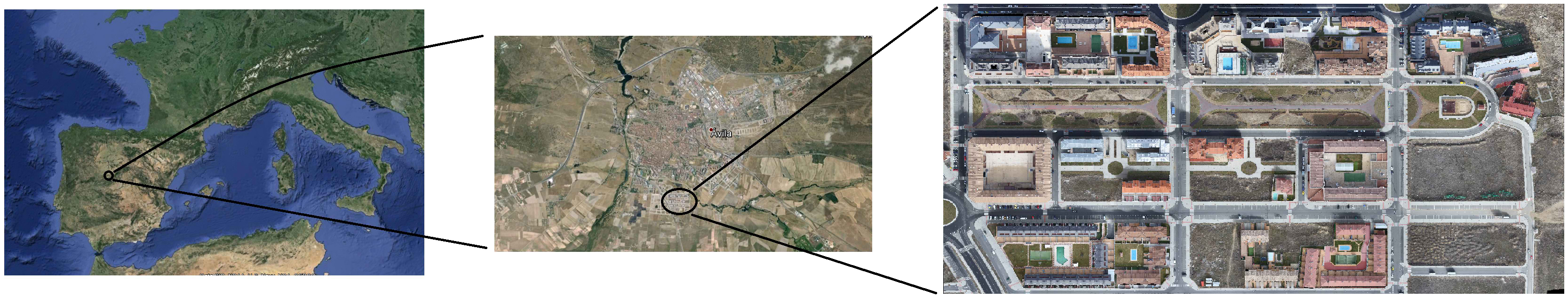
Fig. 1. Location of the area chosen as case of study within Spain, and orthophotograph of the neighborhood.
The city of Ávila was chosen to its climate, which is continental Mediterranean. This implies that the temperature differences between summer and winter are very high, up to 30ºC, and that rain is scarce. This makes building materials suffer a wide range of temperatures, with the consequent reactions of contraction and expansion that could cause fissures and deformation.
The area chosen is a neighborhood built in the last 10 years, so the envelope consists on a structure of reinforced concrete, with double layer of brick and an inner insulation camera (insulation layer plus cavity wall). These buildings should not present a bad thermal behavior, unless for the possible presence of thermal bridges and for the bad installation if the insulation system. On the other hand, the neighborhood is inhabited by young families and students, which are the ideal fraction of inhabitants for being subjected to energy studies, due to their a-priori interest in energy efficiency and new technologies.
2. Thermographic mobile mapping unit
The Thermographic Mobile Mapping Unit, shown in Fig. 2, has been designed for the joint acquisition of geometric 3D data and thermographic data of big-scale areas, especially focused on urban areas, where the combination of these types of information is essential for a wide variety of applications, from condition of infrastructural elements (pavement, road) to energy behavior of buildings. The platform chosen for the development of the prototype is a Mercedes Vito van (Fig. 2), but the same procedure can be applied from any other wheeled vehicle.
Figure 2
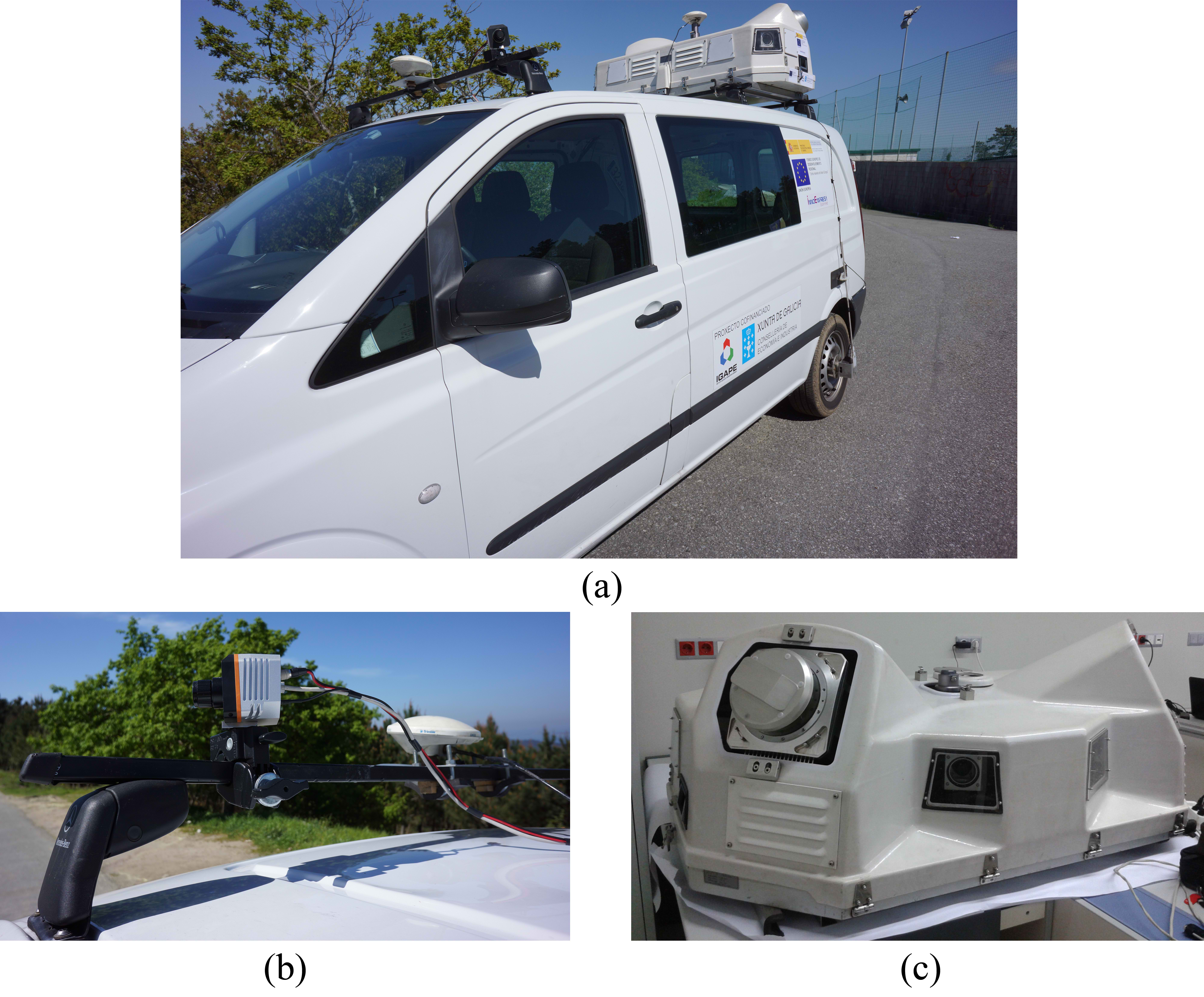
Fig. 2. (a) Thermographic Mobile Mapping Unit. (b) Scanning system. (c) Thermographic camera.
The Thermographic Mobile Mapping Unit consists on a scanning system from Optech, and a thermographic camera from Xenics. The scanning system is formed by 2 scanning heads, placed diagonally to the direction of the vehicle in such way that the union of the measurements of the two heads measures plane coordinates of all the points in 360º. It also includes a GNSS (Global Navigation Satellite System) sensor for positioning the vehicle in the global coordinate system; this way, the position of the vehicle, and consequently of the sensors at every moment during acquisition is known. In order not to limit the movement speed of the Thermographic Mobile Mapping Unit, the scanning frequency of the LiDAR sensors is set to 150 Hz, so they generate 2D profiles of points. Each profile has a system position datum associated, in such a way that the positioning of each profile on the trajectory supplies the third coordinate to the points, thus making possible the posterior generation of the 3D point cloud.
However, the reception of satellites by the GNSS sensor is not always guaranteed in urban environment, especially when travelling through narrow urban canyons. For this reason, an IMU is also integrated in the unit, (Inertial Measurement Unit). This sensor is formed by three accelerometers, three gyroscopes and a pressure sensor, measuring the rotation of the vehicle during its displacement in the three angles (yaw, pitch, and roll, or turns in the x, y, and z axis, respectively). The measurements of this sensor allow the interpolation of the trajectory of the vehicle between positions measured by the GNSS sensor, thus completing those positions where the satellite reception is lost. More information of the scanning system can be found in [21].
Regarding thermal information, the thermographic camera is integrated in the system on a front position, looking at the buildings in front of the vehicle, with a 45º angle regarding the advance direction, either to the left or to the right depending on the façade under study and the allowed direction of circulation in the road under inspection (Fig. 3). The position is chosen in order to increase the field of view minimizing the angle effect in the measurements of temperature [22]. The model used is Gobi384, from Xenics, which presents an Uncooled Focal Plane Array of 384 x 288 microbolometers. The thermographic lens has a focal length of 10 mm, implying a Field of View of 50º × 40º (3 × 3 m at a distance of 3 m between camera and target). The maximum acquisition rate of the camera is 20 images per second, and this is the rate chosen for the acquisition from the vehicle, avoiding the loss of information during displacement, and keeping individual images stable, with no blur effect. Each image is associated to a position in the trajectory (Fig. 4), which allows its georefenciation and later positioning in the point cloud.
Figure 3
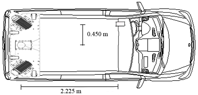
Fig. 3. Schematic figure of the Thermographic Mobile Mapping Unit, with distances between the thermographic camera and the scanning system.
Figure 4
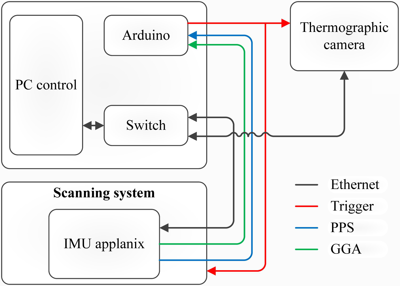
Fig. 4. Synchronization of the scanning system with the thermographic camera: the positioning system sends the time to the control PC and to the Arduino microprocessor. When the time interval is reached, the Arduino sends a trigger to the thermographic camera for the acquisition of an image. Images are sent to the control PC via Ethernet, where they are stored together with their corresponding time stamp from the positioning system. This way, thermographic image and position in the trajectory are associated via the time stamp.
In order to allow further correction of ambient and surface parameters, the thermographic information is saved in .XVI format, developed by Xenics, the camera manufacturer. This format stores images in a single file, similar to a video, but allowing access to the temperature matrices of each image.
One especial characteristic of the camera is its geometric calibration, implying in this case the knowledge of its interior orientation parameters, and of its exterior orientation parameters with respect to the scanning device. Both sets of parameters are shown in Tables 1 and 2, and their knowledge allows the correction of the distortion in the images as well as the correct positioning of each image in the point cloud.
Table 1
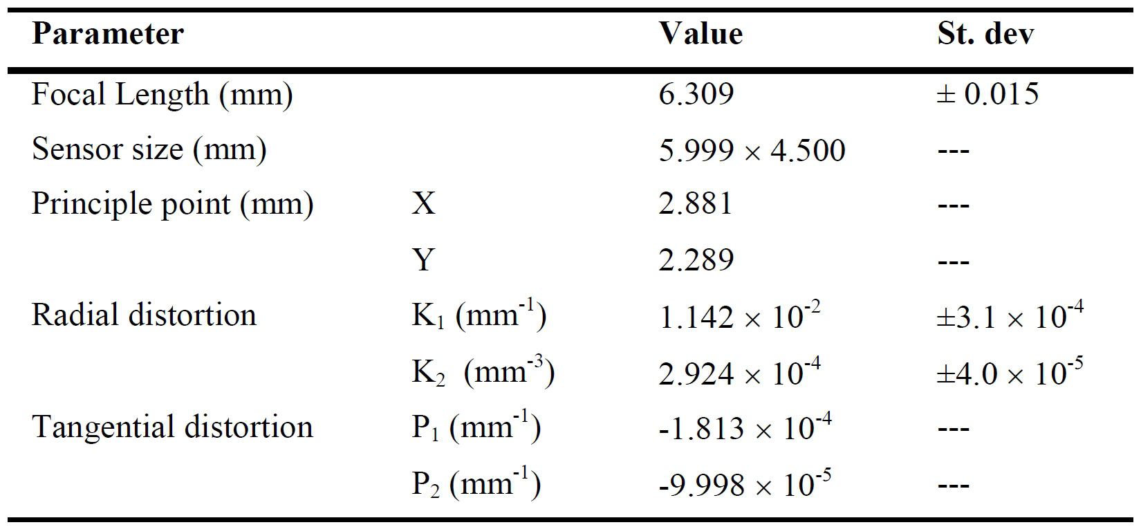
Table 1. Interior orientation parameters of the thermographic camera in the thermographic mobile mapping unit.
Table 2
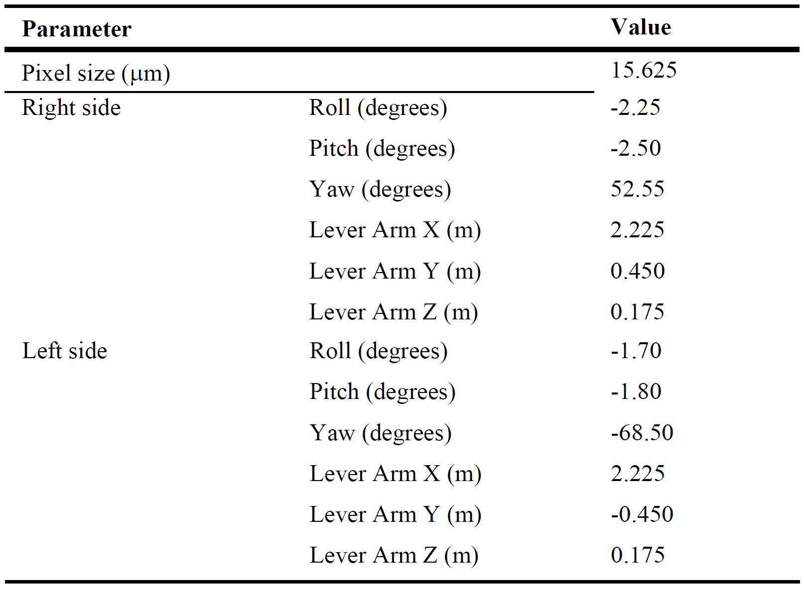
Table 2. Exterior orientation parameters of the thermographic camera with respect to the scanning device.
The Thermographic Mobile Mapping Unit in its current configuration allows the acquisition of geometric and thermographic data of big areas at high speed. As an example, a neighborhood of 157.000 m2 can be inspected in only 1 hour, involving the acquisition of geometric data (trajectory and point clouds) in 9 strips in addition to the 9 corresponding thermographic image sequences, each of them with more than 300 images.
3. Generation of thermographic 3D point clouds
The generation of thermographic 3D point clouds from the data acquired with the Thermographic Mobile Mapping Unit implies a procedure with three different steps: generation of the 3D point clouds from the data acquired with the LiDAR, the GPS and the IMU sensors; thermographic image georeferenciation; projection of thermographic images on the 3D point cloud (Fig. 5). These steps will be explained in detail in the following paragraphs.
Figure 5
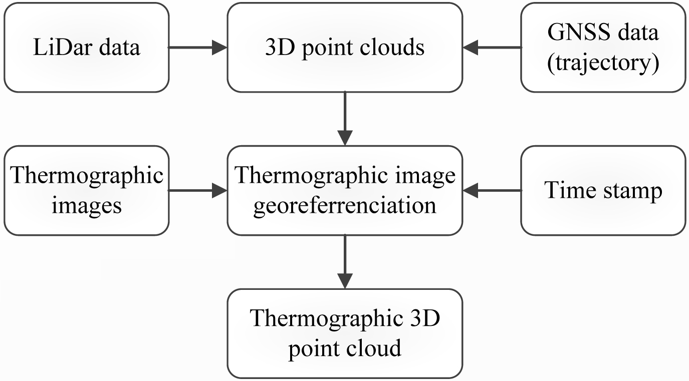
Fig. 5. Flow diagram for data processing towards the generation of thermographic 3D point clouds.
First, the trajectory followed by the Thermographic Mobile Mapping Unit is calculated using the GPS and IMU data, and then corrected using the closest GPS base for reference. The trajectory is saved to a SBET file (Smoothed Best Estimate of Trajectory), consisting on a high precision positioning solution. The SBET file contains data about the GPS time, distance travelled in the inspection, geographical and UTM coordinates, orientation and speed in each spatial coordinate.
The calculated trajectory followed by the Thermographic Mobile Mapping Unit, together with the position data of each scanning head relative to the origin of coordinates are fused together with the point clouds acquired with the LiDAR sensors, using the timestamps transferred by the GPS. This step is performed using DASHMap software by Optech©, provider of the scanning system. The 3D point clouds are presented in .LAS format (LASer file format, a public binary file format approved by the American Society for Photogrammetry and Remote Sensing, ASPRS), chosen for its capability for exchange of LiDAR data from different sensors, Fig. 6.
Figure 6
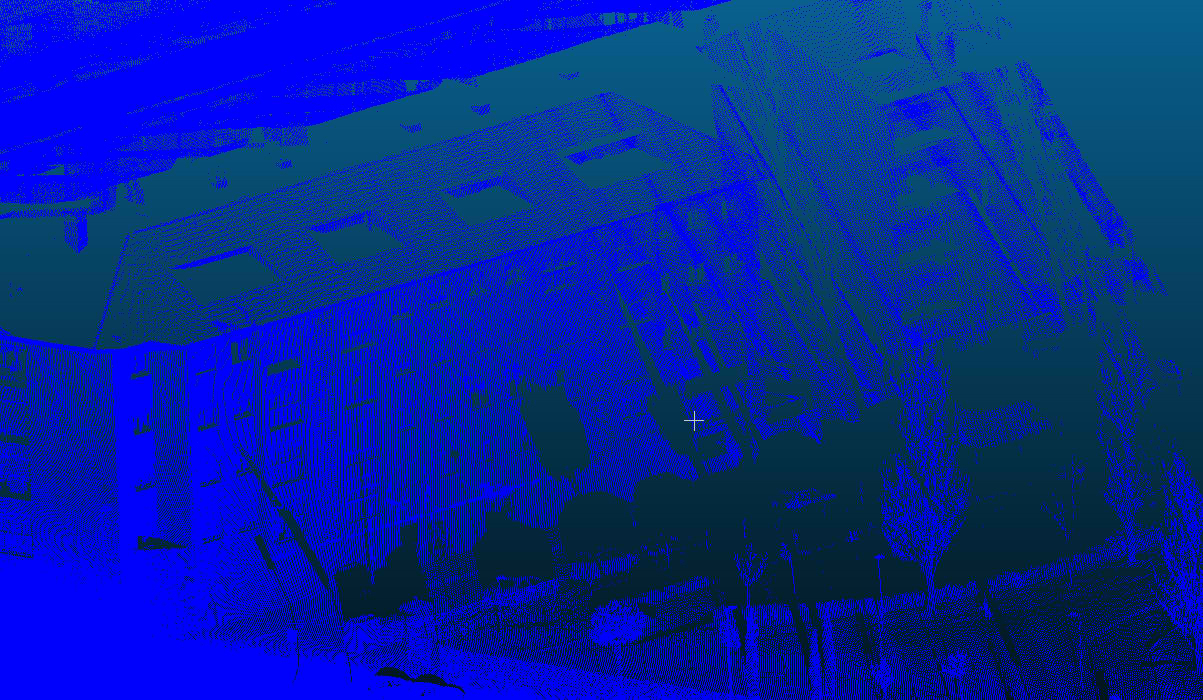
Fig. 6. 3D point cloud generated from the combination of positioning and scanning data.
Processing of the thermographic data can be performed in parallel. The first step of this process is the conversion of each image, from its matrix with temperature values, to a matrix with grey values, where each position becomes the corresponding pixel value. Then, each value is given a color according to a color palette and the existing temperature interval; it is recommended to choose a unique temperature interval for the representation of all the thermographic images. This way, comparisons can be made between buildings, and automatic temperature segmentation of the point clouds can be implemented for all buildings with the same configuration [23]. This way, thermographic data is transformed from mathematical matrices to image files (Fig. 7).
Figure 7
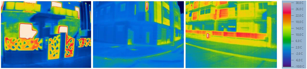
Fig. 7. Processed thermographic images, ready for being projected on their corresponding positions in the point cloud.
Since each thermographic file has associated a point in the trajectory, and the position of the camera with respect to the origin of coordinates is known, each set of pixel values is projected into their corresponding positions in the point cloud. This step is performed using the tool provided by Lynx Software® for the projection of RGB images into the point clouds. The fact of projecting thermographic images requires the generation of a trajectory file compatible with the software, which implies that the trajectory file should contain certain parameters such as focal distance of the lens, orientation and position of the thermographic camera respecting the origin of coordinates in the Scanning System, and the time stamp of each position (Fig. 5). The introduction of the interior calibration parameters (Table 1) in the tool allows the correction of the radial distortion introduced in the images by the lens previously to its projection on the point cloud.
Finally, the projection of the pixel values on the point clouds results in thermographic 3D point clouds. This step is based on the perspective projection of each image into the point cloud (Eq. (1)). Since all the parameters are known in advance thanks to the orientation of the camera and the generation of the 3D point clouds using GPS coordinates, this step does not require the performance of any iteration. Consequently, image projection is an efficient step, only limited by the number of points existing in the point cloud and the number of thermographic images to be projected. For this reason, the speed of the process is exclusively dependent of the computer used, and its storage and computing capacities.
where [d]=[dx,dy,dz] is the 2D position of a point in the image, dz is equal to the focal length of the camera (Table 1), R is the rotation matrix defined by the orientation of the camera with respect to the positioning system, which is established as reference of coordinates. The rotation angles are given in Table 2, [a]=[ax,ay,az] is the 3D position of a point subjected to projection, and [c]=[cx,cy,cz] is the 3D position of a point representing the camera.
The final product allows the visualization of the thermal information over the geometric information, providing complete data in a practical and easy-to-use format to the building inspector for the evaluation of the buildings in the area.
4. Energy-related studies in urban environment
The generated thermographic 3D point clouds are products that stand the performance of thermographic analysis, detection and interpretation of thermal faults, as well as geometric measurements such as the length of the thermal bridges. Some examples are shown in Figs. 8–11, corresponding to a case study performed for testing both the system and the methodology. Analysis can be performed both on a qualitative and on a quantitative basis; for this reason, qualitative evaluations are given in every figure caption, whereas a short quantitative analysis is performed for Fig. 8.
Figure 8

Fig. 8. Detail of a thermographic point cloud, where the severe heat loss through the windows and the elevator shaft is clearly visible due to the high temperature of the surface (in red).
Figure 9
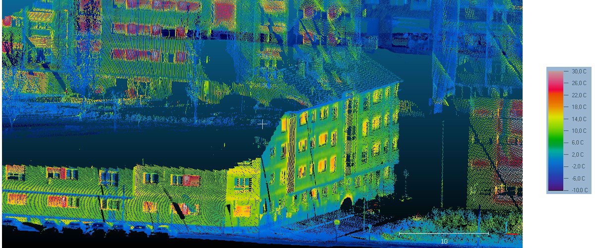
Fig. 9. Detail of thermographic point cloud, focusing on a building with noticeable thermal bridges in the union between floor slabs and the main façade, due to their high temperature (in yellow) in comparison with the façade.
Figure 10
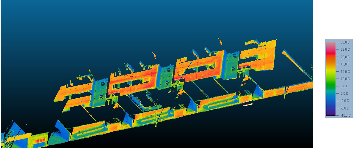
Fig. 10. Detail of thermographic point cloud, oblique aerial view. A lack of insulation is detected in this set of buildings, due to the higher temperature of the main façades (in orange) which are in contact with heated indoor spaces, with respect to the stairs shafts (in blue). What is more, the contacts between floor slab and interior walls and the façade (in red), are areas where heat is easily lost, thus constituting thermal bridges.
In the case that interest is on the performance of quantitative studies, the first step consists on the correction of the temperature values in the thermographies, taking into account the emissivity value of the different materials present in the image. The emissivity values can either be extracted from tables published by different thermographic organizations [24], or calculated through a simple emissivity test. The emissivity test consist on the measurement of the real surface temperature with a contact thermometer and the computation of the emissivity value using the real and the thermographic temperatures, and Stefan-Boltzmann’s law (Eq. (2)):
where εrb is the emissivity value of the “Real Body”, Trb is the temperature of the “Real Body”, measured with the contact thermometer, Tbb is the temperature of the “Black Body”, extracted from the thermographic images.
Another option would be the performance of the emissivity test based on the black tape as in [25], which is a more limited approach given the need of placing tape in every surface, in addition to acquire images where the tape appears and is clearly distinguishable.
The building in Fig. 8 suffers an important energy loss through the elevator shaft, which can be quantified using the information included in the thermographic 3D point cloud: surface temperature of 2ºC, area of heat transmission 19 m2. Ambient conditions during data acquisition were 6ºC and 40% RH. The configuration of the construction is known, as mentioned in section 1.1 (double-brick layer, insulation layer consisting on insulation plus cavity wall), allowing the computation of the transmission coefficient for the envelope, also known as U-value. Consequently, using the formula for heat transmission (Eq. (3)), with a U-value of 0.52 W/m2K, leads to a heat loss through the elevator shaft of 166.4 W:
Regarding the case of study, the complete thermographic 3D point cloud is constituted by 35,514,404 points, unevenly distributed in an area of 157.000 m2. This distribution is caused by the measuring range of the Thermographic Mobile Mapping Unit, since the upper part of the façades and the roofs cannot be measured with it from the floor. An aerial view of the complete point cloud is shown in Fig. 12. What is more, time saved with respect to a current energy inspection is significant, especially taking into account that the products are not comparable: Table 3.
Figure 11
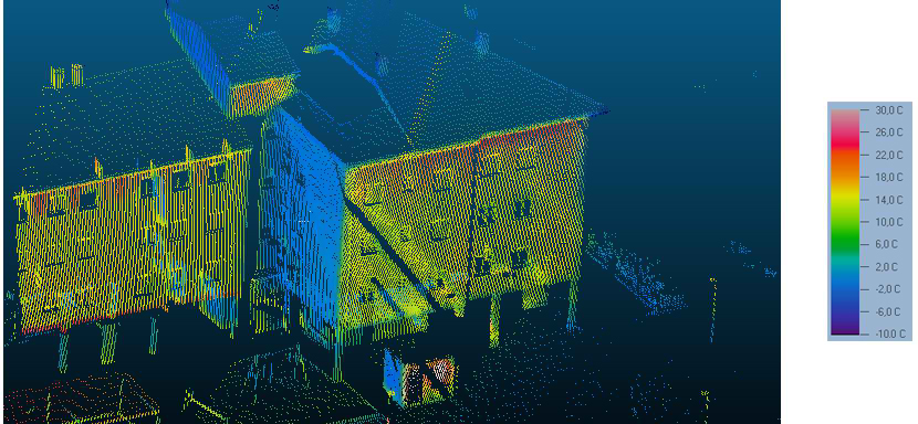
Fig. 11. Detail of thermographic point cloud where the heat accumulation in the upper parts of the building can be detected due to the progressive temperature pattern: from lower temperatures (blue, green) to higher temperatures (orange, red).
Figure 12
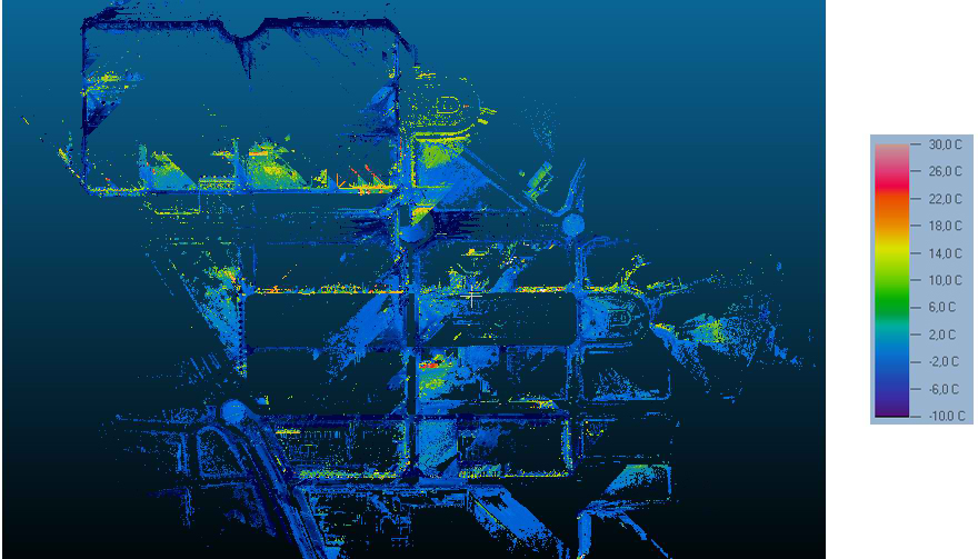
Fig. 12. Aerial view of the thermographic point clouds generated from the area case of study.
Table 3
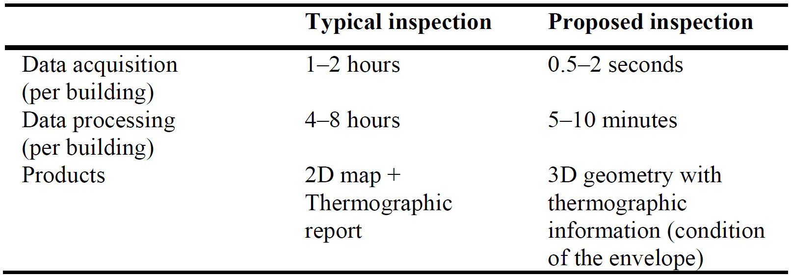
Table 3. Comparison of time needed for the different processes involved in energy audits, and products obtained. Time intervals are given, due to the complexity of stating absolute values (which depend on the dimension of the building, and the computing capacity of the PC used for data processing).
5. Conclusions
This paper presents a methodology for the generation of thermographic 3D point clouds of buildings, in an automatic way and implying short time-consumption for the inspection of several buildings in the same area. The Thermographic Mobile Mapping Unit mounted for this task is described, along with its sensors. Data acquisition and processing procedures are explained. Finally, some examples of the capabilities of the methodology are shown.
The main contribution of the presented methodology is the availability of three-dimensional geometric information of the buildings together with the thermographic data, allowing the detection of faults in a fast and easy manner for the building inspector. In addition, the methodology stands the acquisition of data from several buildings in the same inspection, speeding the process as well as widening the inspections possible: individual building inspection looking for thermal faults; quantification of natural light available in each building, and each floor of the building, regarding the shading buildings and obstacles [5,13]. The latter can also be useful for the analysis of glare problems (both disability and discomfort), given that the 3D point cloud of all buildings is available, and can be used for the analysis of the trajectory of light rays using software such as Ecotect from Autodesk©. Regarding group analysis, thermal inertia of building groups can be studied, as well as detection of heat islands within one urban area and identification of the building in the most severe need of intervention, among others. What is more, the presented methodology stands as a big advance in the field of energy studies, which are currently performed building by building, maybe using a thermographic camera but with the only geometric support of the construction plans (if existing) or a laser distance-meter. In addition, and comparing to current energy inspections based on energy bills, the methodology presented allows the identification of the areas where energy is more wasted than used, both within each building and within the neighborhood.
Although the methodology can be accused of missing detail information of some parts of buildings, the detail provided is more than enough for the main applications of the methodology: detection of thermal faults with a certain significance to the building, study of the thermal performance of buildings in a group, and thermal behavior of the urban area. On the other hand, the traditional method allows the operator to focus on the most interesting elements, while the camera in the Thermographic Mobile Mapping Unit is fixed on top of the vehicle, which prevents it from moving.
In order to increase the automation and utility of this methodology, for example for energy rehabilitation management, future work will deal with the development of algorithms for the automatic detection of heat leakages, moisture and cracks on the thermographic 3D point clouds. Another interesting issue is the use of the knowledge of the geometry of the building and the surface of its roof for evaluating the optimal placement of PV (photovoltaic panels). Apart from the computation of potential areas for PV installation, the thermographic 3D point clouds can establish the areas with the littlest shading projected by the surrounding buildings (since the height of the different buildings is available) [26]. In addition, thermographic 3D point clouds can provide information about the most favorable buildings regarding solar radiation, given the temperatures reached in their upper part (due to the Sun and not to the accumulation of hot air in the upper part of the building, indoors.
Acknowledgments
Authors would like to give thanks to the Consellería de Economía e Industria (Xunta de Galicia), Ministerio de Economía y Competitividad and CDTI (Gobierno de España) for the financial support given through human resources grants (FPDI-2013-17516), and projects (IPT2012-1092-120000, ITC-20133033 and ENE2013-48015-C3-1-R). All the programs are cofinanced by the Fondo Europeo para el Desarrollo Regional (FEDER).
Contributions
H. Lorenzo Cimadevila conceived the study. J. Martínez Sánchez and D. Roca Bernárdez integrated the sensors and performed data acquisition. J. Cereijo García performed the data processing, S. Lagüela López analyzed the data, and the two of them wrote the manuscript.
References
- M. Murray, N. Finlayson, M. Kummert, J. Macbeth, Live Energy TRNSYS – TRNSYS simulation within Google Sketchup, in: Building Simulation 2009, 2009, pp. 1389–1396, Glasgow, Scotland. http://www.ibpsa.org/proceedings/BS2009/BS09_1389_1396.pdf
- M. Kedzierski, A. Fryskowska, Terrestrial and Aerial Laser Scanning Data Integration Using Wavelet Analysis for the Purpose of 3D Building Modeling, Sensors 14 (2014) 12070–12092. http://dx.doi.org/10.3390/s140712070
- K. Einar Larsen, F. Lattke, S. Ott, and S. Winter, Surveying and digital workflow in energy performance retrofit projects using prefabricated elements, Automation in Construction 20 (2011) 999–1011. http://dx.doi.org/10.1016/j.autcon.2011.04.001
- C. Wang and Y. Cho, Automated 3D building envelope recognition from point clouds for energy analysis, in: Construction Research Congress, 2012, pp. 1155–1164.
- L. Díaz-Vilariño, S. Lagüela, J. Armesto, and P. Arias, Indoor daylight simulation performed on automatically generated as-built 3D models, Energy and Buildings 68 (2014) 54–62. http://dx.doi.org/10.1016/j.enbuild.2013.02.064
- C.A. Balaras and A.A. Argiriou, Infrared thermography for building diagnostics, Energy and Buildings 34 (2002) 171–183. http://dx.doi.org/10.1016/S0378-7788(01)00105-0
- E. Rosina and J. Spodek, Using infrared thermography to detect moisture in historic masonry: a case study in Indiana, APT Bulletin 34 (2003) 11–16. http://dx.doi.org/10.2307/1504847
- P. Bison, A. Bortolin, G. Cadelano, G. Ferrarini, L. Finesso, F. Lopez, and X. Maldague, Evaluation of frescoes detachments by partial least square thermography, in: QIRT 2014, 2014, Bordeaux, France.
- D. A. Vanocker, E. M. Johnson, and T. D. Marcotte, The identification of corrosion-related damage from cramp anchors in a limestone-clad building façade using NDE techniques, Journal of ASTM International 4 (2007) 35–46. http://dx.doi.org/10.1520/JAI100875
- A. Bortolin, G. Cadelano, G. Ferrarini, P. Bison, F. Peron, and X. Maldague, High resolution survey of buildings by lock-in IR thermography, in: Thermosense: Thermal Infrared Applications XXXV, 2013, Baltimore, USA. http://dx.doi.org/10.1117/12.2016592
- S. Lagüela, L. Díaz-Vilariño, J. Martínez, and J. Armesto, Automatic thermographic and RGB texture of as-built BIM for energy rehabilitation purposes, Automation in Construction 31 (2013) 230–240. http://dx.doi.org/10.1016/j.autcon.2012.12.013
- M. Previtali, L. Barazzetti, V. Redaelli, M. Scaioni, and E. Rosina, Rigorous procedure for mapping thermal infrared images on three-dimensional models of building façades, Journal of Applied Remote Sensing 7 (2013) 073503. http://dx.doi.org/10.1117/1.JRS.7.073503
- L. Díaz-Vilariño, S. Lagüela, J. Armesto, and P. Arias, Semantic as-built 3D models including shades for the evaluation of solar influence on buildings, Solar Energy 92 (2013) 269–279. http://dx.doi.org/10.1016/j.solener.2013.03.017
- M. Van Esch, R. Looman, and G. de Bruin-Hordijk, The effects of urban and building design parameters on solar access to the urban canyon and the potential for direct passive solar heating strategies, Energy and Buildings, 47(2012) 189–200. http://dx.doi.org/10.1016/j.enbuild.2011.11.042
- F. Asdrubali, A. Presciutti, and F. Scrucca, Development of a greenhouse gas accounting GIS-based tool to support local policy making – application to an Italian municipality, Energy Policy, 61 (2013) 587–594. http://dx.doi.org/10.1016/j.enpol.2013.05.116
- H. Takebayashi and M. Moriyama, Relationships between the properties of an urban street canyon and its radiant environment: Introduction of appropriate urban heat island mitigation technologies, Solar Energy 86 (2012) 2255–2262. http://dx.doi.org/10.1016/j.solener.2012.04.019
- J. Wei, J. He, Numerical simulation for analyzing the thermal improving effect of evaporative cooling urban surfaces on the urban built environment, Applied Thermal Engineering 51 (2013) 144–154. http://dx.doi.org/10.1016/j.applthermaleng.2012.08.064
- F. Ramos, D. Siret, and M. Musy, A 3D GIS managing building rehabilitation process, in: Proceedings of the 12th International conference on Geoinformatics Geospatial Information Research-Bridging the Pacific and Atlantic, 2004, Gävle, Sweden.
- M. Previtali, S. Erba, E. Rosina, V. Redaelli, M. Scaioni, and L. Barazzetti, Generation of a GIS-based environment for infrared thermography analysis of buildings, in: Infrared Remote Sensing and Instrumentation XX, 2012, 85110U. http://dx.doi.org/10.1117/12.930050
- L. Hoegner and U. Stilla, Automatic generation of façade textures from terrestrial thermal infrared image sequences, in: the 12th Quantitative InfraRed Thermography Conference, 2014, Bordeaux, France.
- I. Puente, H. González-Jorge, B. Riveiro, and P. Arias, Accuracy verification of the Lynx Mobile Mapper system, Optics & Laser Technology 45 (2013) 578–586. http://dx.doi.org/10.1016/j.optlastec.2012.05.029
- L. Coret, X. Briottet, Y. Kerr, and A. Chehbouni, Simulation study of view angle effects on thermal infrared measurements over heterogeneous surfaces, IEEE Transactions on Geoscience and Remote Sensing 42 (2004) 664–672. http://dx.doi.org/10.1109/TGRS.2003.819443
- D. González-Aguilera, P. Rodríguez-Gonzálvez, J. Armesto, S. Lagüela, Novel approach to 3D thermography and energy efficiency evaluation, Energy and Buildings 54 (2012) 436–443. http://dx.doi.org/10.1016/j.enbuild.2012.07.023
- Omega. Table of total emissivity. Available at: http://www.omega.com/temperature/z/pdf/z088-089.pdf
- P. Fokaides and S. Kalogirou, Application of infrared thermography for the detection of the overall heat transfer coefficient (U-value) in building envelopes, Applied Energy 88 (2011) 4358–4365. http://dx.doi.org/10.1016/j.apenergy.2011.05.014
- I. Ullah, Development of Fresnel-based Concentrated Photovoltaic (CPV) System with Uniform Irradiance, Journal of Daylighting 1 (2014) 2–7. http://dx.doi.org/10.15627/jd.2014.1
Copyright © 2014 The Author(s). Published by solarlits.com.


