Daylight Utilization with Light Pipe in Farm Animal Production: A Simulation Approach

^a Lund University, Institute for Architecture and the Built Environment, Division of Energy and Building Design, Box 118, 221 00 Lund, Sweden.
^b Swedish University of Agricultural Sciences, Department of Biosystems and Technology, Box 103, SE-23053 Alnarp, Sweden.

* Corresponding author. Tel: +46 40 41 54 85
alejandro.pacheco@bau.se (A. P. Diéguez’)
niko.gentile@ebd.lth.se (N. Gentile)
hans.von.wachenfelt@slu.se (H. v. Wachenfelt)
marie-claude.dubois@ebd.lth.se (M.-C. Dubois)

History: Received 12 September 2015 | Revised 10 December 2015 | Accepted 11 December 2015 | Published online 08 January 2016

Citation: Alejandro Pacheco Diéguez’, Niko Gentile, Hans von Wachenfelt, and Marie-Claude Duboisba, Daylight Utilization with Light Pipe in Farm Animal Production: A Simulation Approach, Journal of Daylighting 3 (2016) 1-11. http://dx.doi.org/10.15627/jd.2016.1

Figures and tables

Figure 1
Table 1
Table 2
Figure 2
Table 3
Table 4
Figure 3
Table 5
Table 6
Table 7
Figure 4
Figure 5
Figure 6
Figure 7
Figure 8
Figure 9
Figure 10
Figure 11
Figure 12

Abstract

Light pipes offer a passive way to bring daylight inside deep buildings, such as agricultural buildings. However, the lack of reliable performance predictability methods for light pipes represents a major obstacle preventing their widespread use. This paper evaluates a simulation approach for performance prediction and identifies key light pipe design parameters affecting their daylight transmission performance. The study was carried out through continuous monitoring of daylight in two full-scale, identical pig stables fitted with two light pipe systems, Solatube^® and Velux^®. The experiment included three continuously measuring sensors in each stable and an outdoor sensor during 2013 and 2014. A forward raytracing tool, TracePro^®, was used for illuminance prediction and parametric simulations. The simulation results for overcast skies indicated discrepancies between the simulated and average measurement results below 30% in all cases. The discrepancies for clear skies were somewhat higher, i.e., below 30% for 67% of the cases. The higher discrepancies with clear skies were due to the overestimation of absolute sunlight levels and absence of an advanced and detailed optical characterization of the dome collector’s surface. The parametric results have shown that light pipes’ performance is better during summer time, in sunny climates, at low to mid-latitudes, which provides higher solar altitudes than during winter and cloudy climates at high latitudes. Methods to improve the luminous transmittance for low solar altitudes occurring in Scandinavia include: bending or tilting the pipe, increasing the aspect ratio, improving the pipe specular reflectance, tilting the collector to the south, and using optical redirecting system in the collector.

Keywords

Light pipe; Daylight simulation; Raytracing; Light collector

Nomenclature

τ	Luminous transmittance
Kt	Sky clearness index
Abbreviations
AAD	Average absolute deviation
BSDF	Bi-directional scattering distribution function
CL	Clear sky
OC	Overcast sky
GHI	Global horizontal illumination
LLF	Light loss factor
MLP	Mirror light pipe
ORS	Optical redirect system

1. Introduction

One obvious way to reduce electric lighting consumption is through the optimization of daylight utilization in buildings. Light pipe is one of the light transmission media, which offers a passive way to bring sunlight inside buildings; however, the lack of reliable performance prediction methods is a major obstacle preventing the widespread use of light pipes in buildings. Consequently, the advantages of light pipes cannot be quantified and considered in environmental building design, let alone in modern rating systems like LEED or BREEAM. This paper evaluates a simulation approach to identify key light pipe design parameters and design guidelines and obtain performance predictability, based on illuminance measurements in two pig houses located near Lund, Sweden.

The raytracing technique was first explored by Albrecht Dürer in the 16th century and further developed as research in the 1960s, for computer animations and in the film industry to create photorealistic images and simulate global illumination [1]. Raytracing is a simulation of light rays that are randomly sent in space to predict light levels or create realistic images. The physical context needs to be defined by a model specifying the geometry as well as the optical properties of surfaces defining absorption, reflection, refraction, scattering, and diffraction [2]. Light sources also need to be defined and characterized in the model. The main interest for using raytracing software to simulate complex daylighting systems like light pipes is the capacity to simultaneously handle many more variables than other methods: different locations and sky conditions, diffuser and collector geometry, complex optical properties, and bends in the light pipe [3–6].

Raytracing can be applied either backward or forward. In backward raytracing, the rays are emitted from the end point or point of view and traced back throughout the model to the light sources according to a certain number of light bounces usually 3 to 5 [2]. If light rays hit a light source, the light contribution of that source is added up in the point of view, which means that the accuracy of the results depends on the amount of bounces and rays traced, among other things.

To simulate light pipes, the number of light bounces needs to be increased significantly due to geometrical considerations, with consequent lengthening of simulation times. Moreover, in backward raytracing, the probability of a ray hitting the sun is very low, making it nearly impossible to sample direct sunlight efficiently with this technique [2,7].

In large, low buildings, dominating animal production, windows have a poor core daylighting effect. For growing animals like pigs and poultry, light pipe technology could be an effective way to provide daylight in such buildings. For pig houses, windows or other means of daylight inlets are mandatory according to the Swedish Board of Agriculture regulations [8], and the light requirement for pigs is at least 40 lux for a minimum period of 8 hours per day, as stated by European legislation [9].

The overall aim of this study was to develop a simulation approach allowing the prediction of daylight intensity and distribution in space. The first objective was thus to evaluate the resulting illuminance from daylight through light pipe systems by using a simulation tool and compare these results with measurements in order to obtain performance predictability. The secondary objective was to evaluate key parameters of light pipe design to develop design guidelines. This second objective was achieved by parametric simulations. The hypothesis was that light pipe illumination intensity and light distribution could be assessed and designed by using a simulation tool.

The remainder of this paper is organised as follows. Section 2 describes the selection and description of raytracing method including building a virtual model, defining light sources, pupils and sensor setting, error sources, and a parametric study of key factors for light pipe design. The results are reported in Section 3. In Section 4, the variability of measurements, correspondence between measurements and simulation results, and the parametric study are discussed and compared with respect to the two light pipe systems, and a critical analysis of the data collection method used along with design considerations are presented. In Section 5, conclusions are presented.

2. Materials and methods

The pig houses are located at Odarslöv (55°45'N, 13°15'E) Sweden. The light pipes in house 1, on the eastern side (Velux Sun Tunnel^®), had a bend in connection with a flat collector, while the pipes in house 2, on the western side (Solatube Brighten Up^®), were straight and had a dome collector equipped with a reflector to redirect low-angle sunlight. The pipes were installed on a pitched roof with a 22º-tilt angle, facing approximately north-south, with half the light pipes in each house located on the southern pitch and the other half on the northern pitch. The skies at the site are predominantly overcast in the winter and mixed in the rest of the year. Midday solar altitude ranges from 11º on December 21 to 58º on June 21. The description of houses, light pipes, and measuring system are described in [10].

2.1. Selection of raytracing method

Forward raytracing was selected because of its simplicity, accuracy, capacity to handle the direct sun contribution, and its capacity to simulate large amounts of light bounces within reasonable simulation times. Forward raytracing sends rays from the light sources and through multiple bounces in the virtuel model to determine illumination on a point. At each interaction with the model, rays can be subject to absorption, reflection, refraction, diffraction, and scattering. As the rays spread through the model, the program keeps track of the optical flux associated with each ray [11].

The program used in this study was TracePro^® Expert 7.4.1 [12], equipped with a solar emulator allowing to simulate direct sunlight as well as diffuse light from a variety of sky types. The solar emulator ability to simulate large amounts of light bounces keeping reasonable simulation times, was obtained by simulating only rays directed towards the openings, pupils, or ports of the virtual model of the building.

2.2. Description of the simulation method

2.2.1 Building the virtual model

Raytracing was applied using three steps: building the virtual model, defining the light sources, and defining the pupils and sensors. The virtual model included room envelope, pens partitions, and pen covers, as shown in Fig. 1. Pig feeding systems and several pipes hanging from the ceiling were excluded from the model. This might entail some error in the simulation results, but given the size and position of the omitted elements with respect to the sensors the error should be negligible. The 3D models of the stables were modelled using Rhinoceros^®, and then exported to TracePro^® through an ACIS (*.sat) file. Light pipes were modeled as accurately as possible including the collectors, MLP, and diffusers.

Figure 1

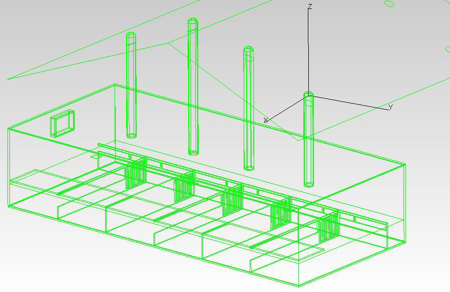
Fig. 1. TracePro^® model of one of the pig houses.

In defining the light sources, the optical properties of the modelled elements were specified in the program to account for the light interactions with these elements. For a complex optical systems like ORS, a goniophotometric specification is required through a BSDF file. This information was provided by the manufacturer for the Velux diffuser and was introduced in the program using the BSDF Converter utility of TracePro^®. The rest of the transparent elements in the light pipes were defined using the fraction of luminus absorptance and transmittance (Table 1), and this information was provided by the manufacturers. For the Velux flat collector, this information was sufficient to characterize it. But for the dome collectors and diffusers of the house 2 light pipes, the information was insufficient to accurately reproduce their interaction with light. Instead, a standard diffuser surface property from the program library was applied to the house 2 diffuser since the BSDF was not available at the time of performing the simulations.

Table 1

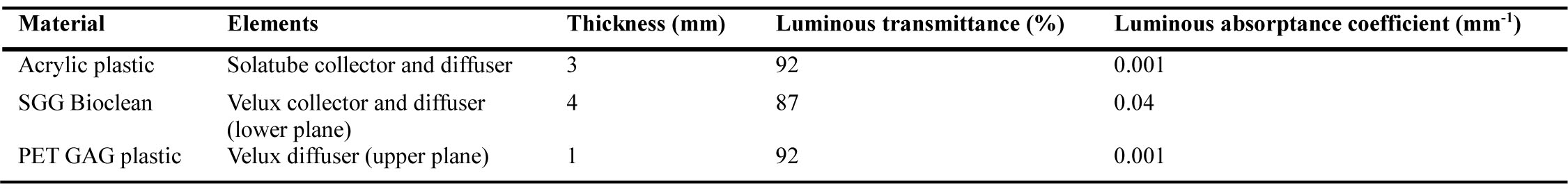
Table 1. Optical characterization of the translucent and transparent materials in TracePro^®.

The reflectance of the other elements included in the model (walls, floor, etc.) was specified, and all the elements in the stables were treated as Lambertian reflectors, i.e., the reflectance data previously measured was introduced as being 100% diffuse (Table 2) [13,14]. This is a common simplification that normally does not introduce significant errors. The MLPs, however, require a more detailed characterization, specifying separately diffuse and specular reflectance.

Table 2

Measured light reflectance of surfaces in the pig houses. A matt white disc whose reflectance was accurately known and a luminance meter were used to measure the reflectance of the different surfaces in the pig houses according to [13] in [14].

Table 2. Measured light reflectance of surfaces in the pig houses. A matt white disc whose reflectance was accurately known and a luminance meter were used to measure the reflectance of the different surfaces in the pig houses according to [13] in [14].

2.2.2 Defining the light sources

The solar emulator utility of TracePro^® was used to simulate daylight from both the sky dome and the sun. Latitude, longitude, date, time, time zone, north vector, and zenith vector needed to be specified to locate the sun position and sky luminance distribution in relation to the model.

The sky luminance distribution is determined by selecting data from a catalogue of predefined sky models. In this case, the overcast and clear skies of the Igawa all-sky models [15], with a range of 50000-80000 rays, were used in the different simulations since they provided a sufficient amount of rays to reach accurate results.

The solar model is also defined by a solar constant expressed in W/m2. The default value (1,067 W/m2) needs to be adapted for each specific location according to elevation and solar altitude. The GHI at sea level according to the solar elevation angle is displayed in Fig. 2(a), and as the city of Lund (closest to Odarslöv) has a low elevation of about 60 m above sea level, it can therefore be assimilated to a place at sea level [16]. The solar constant values introduced in TracePro^® for a place located at sea level were estimated as follows. GHI’s for different solar altitudes on a clear day were simulated in the program. The solar constant was then adjusted for each solar altitude to reach the targeted GHIs, as shown in Fig. 2(a). The resulting values for the solar constant introduced in TracePro^® are plotted in Fig. 2(b). A range of 10000-30000 rays was used in the simulations in order to reach a sufficient level of accuracy.

Figure 2

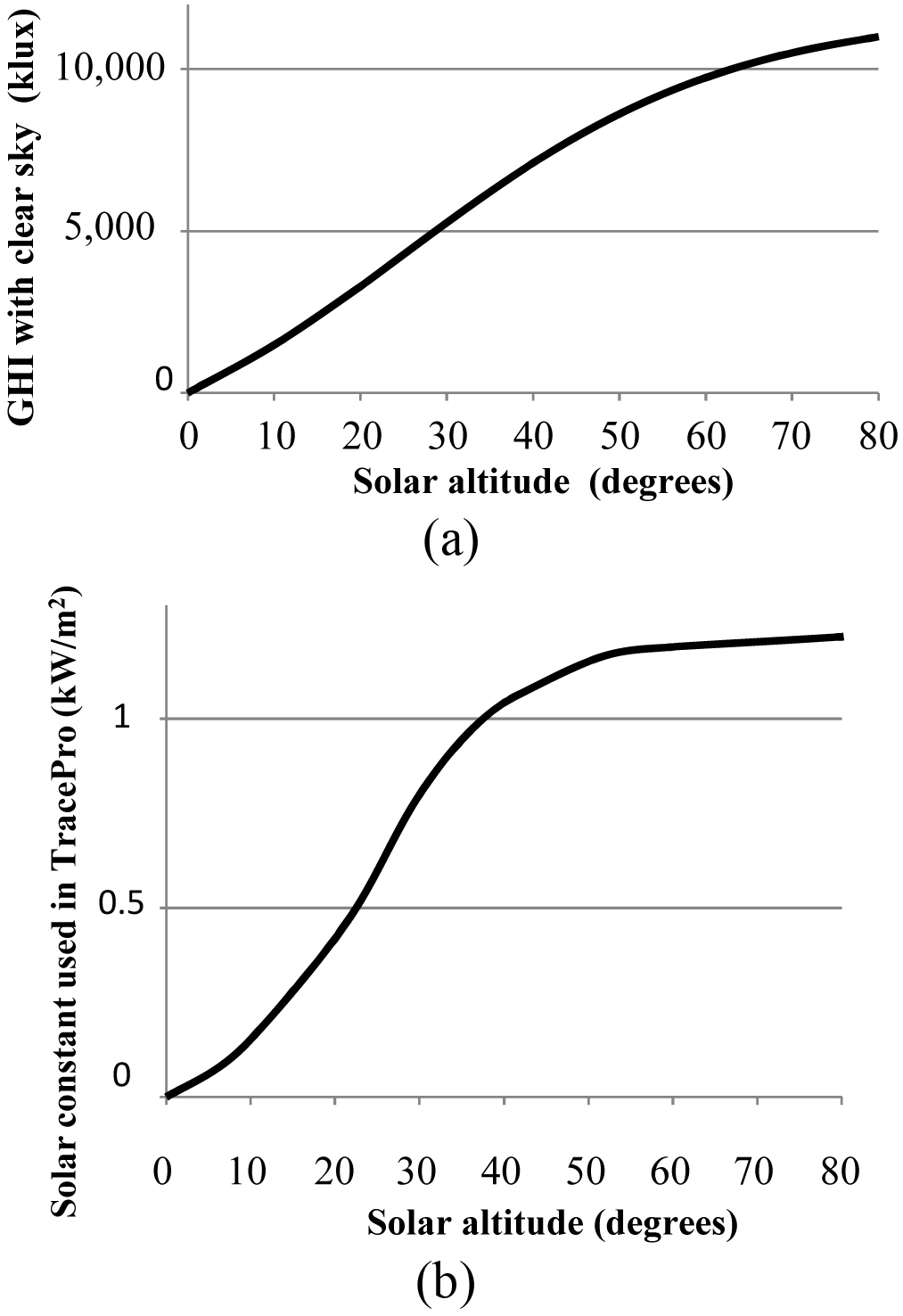
Fig. 2. (a) Horizontal global illuminance with clear sky as a function of solar altitude at sea level [16] and (b) TracePro^® solar constant as a function of solar altitude.

2.2.3 Setting the pupils and sensors

The solar emulator of TracePro^® requires the specification of a pupil and a sensor. A pupil is simply an area close to the entrance of the light rays in the light pipe that is considered in the forward raytracing process while the sensor is the point inside the model where illuminance is ultimately measured. Pupils are surfaces used to reduce the total number of rays going from the light source (the sun or the sky) to the model. The pupil surfaces where the rays are aimed at are placed over the building openings. By casting rays only towards the pupils, the number of simulated light rays are largely optimized, and the simulation time are reduced. It is important to define the location and orientation of the pupils correctly as this can dramatically affect the results and compromise their accuracy. In this case, individual pupils were placed over the exterior apertures of each of the four pipes in each stable. This way the light contribution of each of them on the sensors was considered separately.

The sensors were modelled as 300 mm × 300 mm horizontal squares located in the virtual model in the same position as the sensors used in the measurements. Forward raytracing estimates the illuminance on a surface by adding up the contribution of all light rays meeting that surface. The size of the pupil was considered large enough to be hit by a sufficient amount of light rays so that their value can be averaged to a reasonably accurate value.

2.3. Error sources

This subsection describes the error sources and how the sensor readings and the simulation results were handled to minimize these errors. In total, eleven specific times were picked to compare measurement and simulation results, of which five corresponded to OC and six to CL occurring between December 2013 and March 2014 (Table 3). The data obtained from the measuring system was reliable, still high variability was found in the sensor data averaged every 6 minutes especially with overcast skies. To minimize these fluctuations, three consecutive measurements were averaged in each of the times picked to be compared to the simulation results. The AAD for the measured values was calculated to estimate the variability of light levels at each of the sensors and sky types. This value was expressed as a percentage of the mean of the three measurements according to the following equation

\[ AAD = \frac{\frac{∑(X_n-m(X)}{n}×100}{m(X)} \]

where X_n is the measurement considered, m(X) is mean of the measurement considered, and n is the number of measurements considered (n is 3 in all cases except in OC1 where n is 5).

Table 3

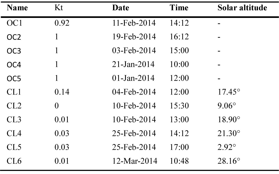
List of times considered for comparing measurement and simulation results, where OC, CL, and Kt stands for overcast, clear sky conditions, and sky clearness index, respectively.

Table 3. List of times considered for comparing measurement and simulation results, where OC, CL, and Kt stands for overcast, clear sky conditions, and sky clearness index, respectively.

The recording measuring system was found to be greatly affected by the amount of soiling in the pig houses as well as the daylight control (on/off) system [10]. A sensor soiling factor (SSF) was determined to account for the accumulation of soiling on the sensors. The sensors were cleaned on the evening of February 11th, i.e., SSF = 0, which was detectable from the sensor readings of the electric light illumination. This reading was the sole source of light, and the window was blacked out. For SSF calculation, the light conditions on February 12 at 09:18 AM were used as reference. This moment was chosen as reference because it had light conditions that occurred every day: the electric lights were on, daylight levels outdoor were low, GHI was 8081 lux, and sensors were clean. A similar situation (lights on and about 8000 GHI) was picked for each of the days considered (Table 4). For each of these days, the SSF was applied to each subsequent reading to correct for the soiling error. The SSF was calculated according to the following equation

\[ SSF_{day~x} = \frac{E_{reference}}{E_{day~x}} \]

where SSF_{day x} is sensor soiling factor on a chosen day, E_reference is illuminance reading from the sensor at the reference moment (February 12 at 09:18; lights on and GHI = 8018 lux), and E_{day x} is illuminance reading from the sensor on the chosen day at a moment when the electric lights were on and the GHI was approximately 8000 lux.

Table 4

Table 4. SSF of the illuminance sensors for each considered time.

With the accuracy in daylight on/off sensor calibration and threshold adjustment, together with the high level of measured daylight variability in space and time, the desired threshold of 40 lux might actually fluctuate.

Only the contributions from light pipes close enough to each sensor to produce a significant output were considered, i.e., lp1 and lp2 for sensors v1 and s1 and light pipes lp2, lp3, and lp4 for sensors v2 and s2. Simulated values were calculated for each of the light pipes individually, and then summed up for each sensor. Contributions from the light pipes that were too far from a sensor were not considered.

The pupils were placed over the collectors of each of the light pipes. This worked well for the flat collector of house 1. For the dome in house 2, a combination of approaches was used to minimize negative side effects, like missing part of the sky rays or large increases in the simulation time.

Generic sky models of clear and overcast skies (Iwaga all-sky model) were used to simulate luminance from the sky dome. The difference in GHI between the actual and simulated sky was adjusted using a correction factor according to the following equation

\[ GHI_{factor} = \frac{GHI_{measured}}{GHI_{simulated}} \]

The measured GHI was obtained from the illuminance sensor located outdoors, while the chosen generic skies were selected according to how close they were to pure overcast or clear skies, i.e., a sky clearness indexes (Kt) closer to 1 or 0, respectively, provided by the Swedish Meteorological and Hydrological Institute for Lund.

2.4. Parametric study

A parametric study was also achieved in order to examine the influence of key parameters of the light pipe design on the overall performance, using the same computer simulation method explained in the previous sections. A starting point (Fig. 3(a) and Table 5) was a small room model, base case, with a light pipe as its sole light source [17]. The simulation was performed for nine variations, i.e., three times (08:00, 10:00, and 12:00) on equinox and solstices (December 21^st, March 21^st, and June 21^st).

Figure 3

(a) Base case TracePro® model, (b) factors affecting the light output from the light pipe, and (c) dependence of the number of reflections in a pipe (aspect ratio 1/11.25) on the zenith angle. Zenith angle = 90 – solar altitude [17].

Fig. 3. (a) Base case TracePro^® model, (b) factors affecting the light output from the light pipe, and (c) dependence of the number of reflections in a pipe (aspect ratio 1/11.25) on the zenith angle. Zenith angle = 90 – solar altitude [17].

Table 5

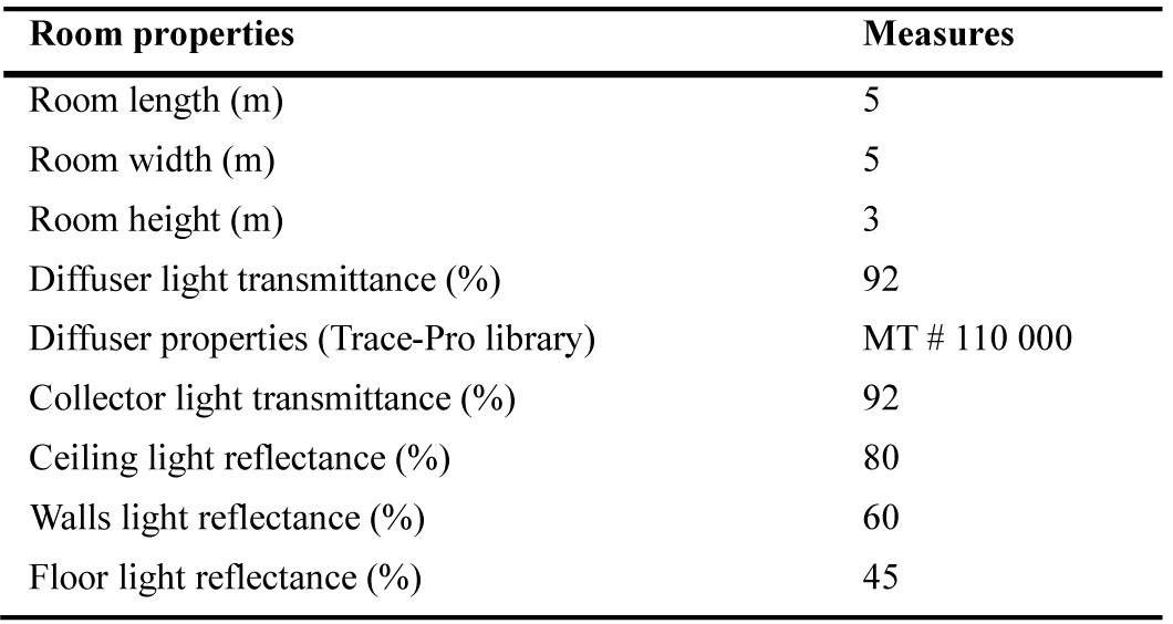
Table 5. Fixed properties for base model in parametric study.

Six parameters were varied (Table 6), and the effect of this variation was analysed and compared to the base case outputs in terms of LLF, illuminance at the diffuser lower surface or illuminance distribution on the floor of the room. The LLF is calculated as the quotient between the exiting light from the diffuser and the incident light on the collector.

Table 6

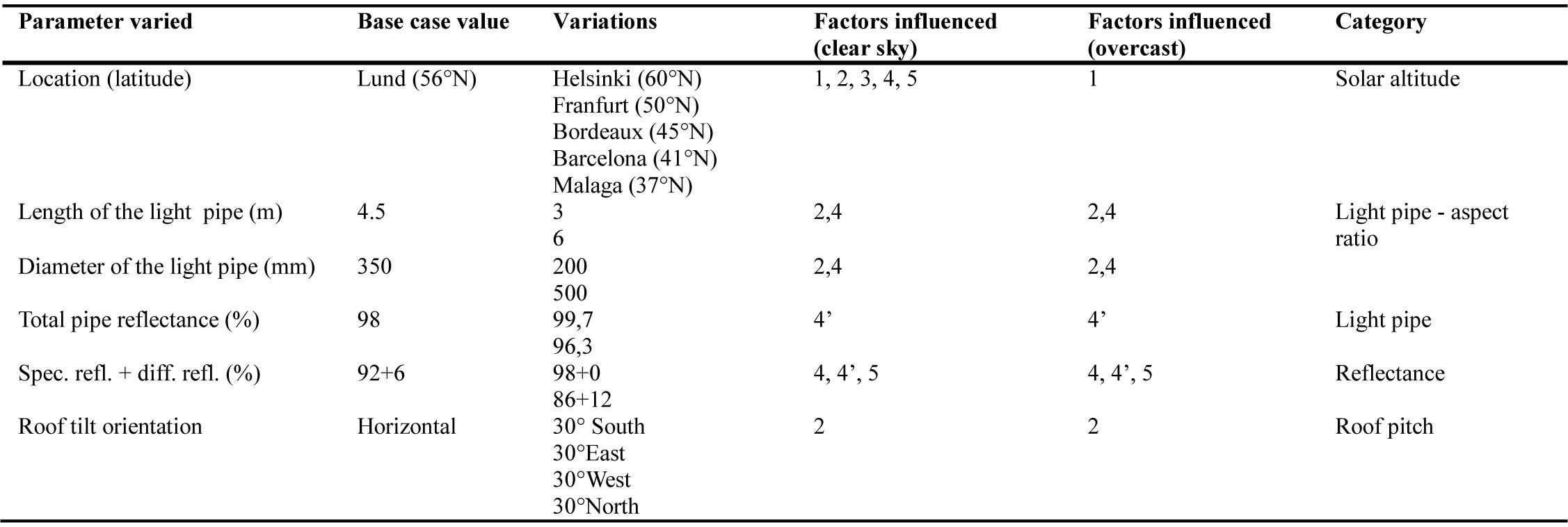
Table 6. Varied parameters, categories, and affected factors.

(1) Amount of light buffered/absorbed by the atmosphere: dependent on the sky clearness and sun position.
(2) Amount of light reaching the collector: depends on the size, shape, location and orientation of the collector.
(3) Amount of light going through the collector: depends on the optical properties of the collector and its position in relation to the incident light rays.
(4) Number of bounces in the light pipe: depends on the direction of the incident light rays (sky clearness and sun position), on the aspect ratio of the light pipe, on the optical properties of the pipe, on geometry of the pipe and on the light deflecting properties of the collector (if any). Figure 3(c) shows how the number of bounces in a given pipe increases exponentially as the sun approaches the horizon.
(4’) Amount of light lost in each bounce: directly linked to the reflectance of the pipe.
(5) Amount of light that goes through the diffuser: dependent on the optical properties of the diffuser, the optical properties and geometry of the light pipe, the redirecting properties of the collector (if any), and the direction of the incident daylight.

3. Results

3.1 Evaluation of the simulation method

The relative difference between simulated and measured illuminance obtained under clear and overcast sky conditions is presented in Table 7.

Table 7

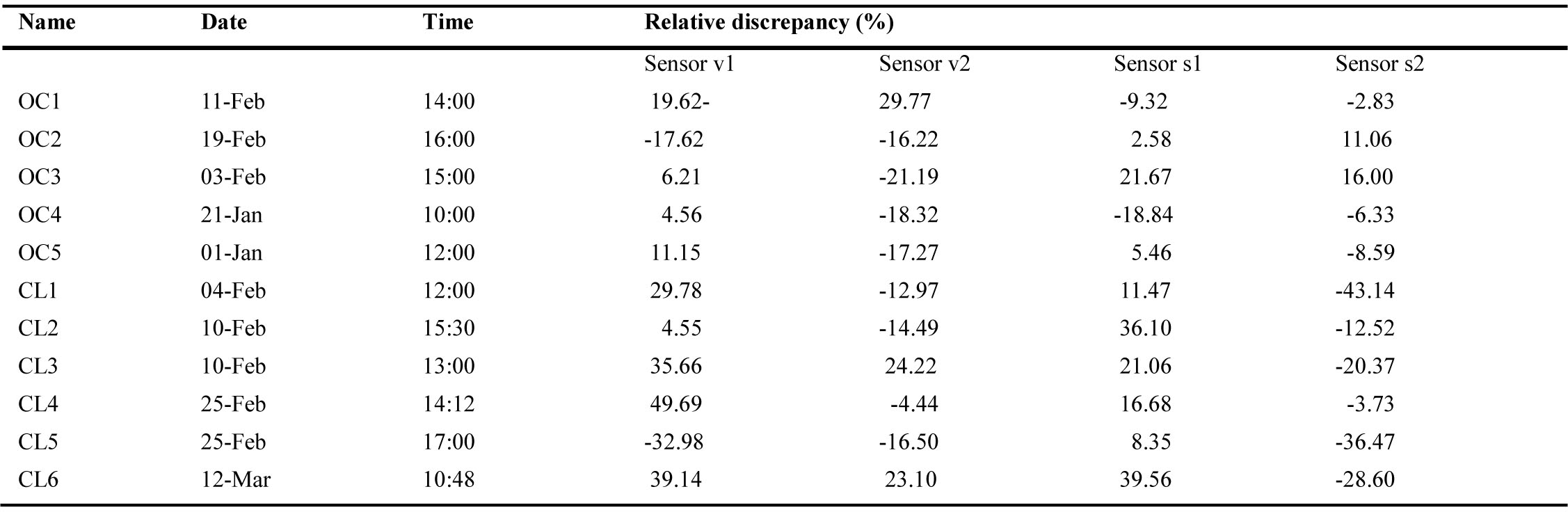
Table 7. Illuminance relative discrepancy of TracePro^® simulation results compared to the measurements.

In general, the overcast skies yield more accurate simulation results compared to clear skies. For overcast sky conditions, the values differed by less than 30% for all cases, less that 20% in 85% of the cases and less than 10% in 40% of the cases. These percentages are lower than for the simulations using clear skies: 67% (<30%), 42% (<20%) and 17% (<10%) respectively, which was an unexpected result.

A graphical representation of measured versus simulated illuminance values for overcast and clear sky conditions is presented in Figs. 4 and 5. The range of measurement values is higher for overcast conditions compared to clear sky conditions. It is also higher for sensors located between two light pipes (v1 and s1) than for sensors located right below the light pipes (v2 and s2), which was an expected result. However, the trend of the measurement results seems to match that of the simulation results for overcast conditions on all sensors.

Figure 4

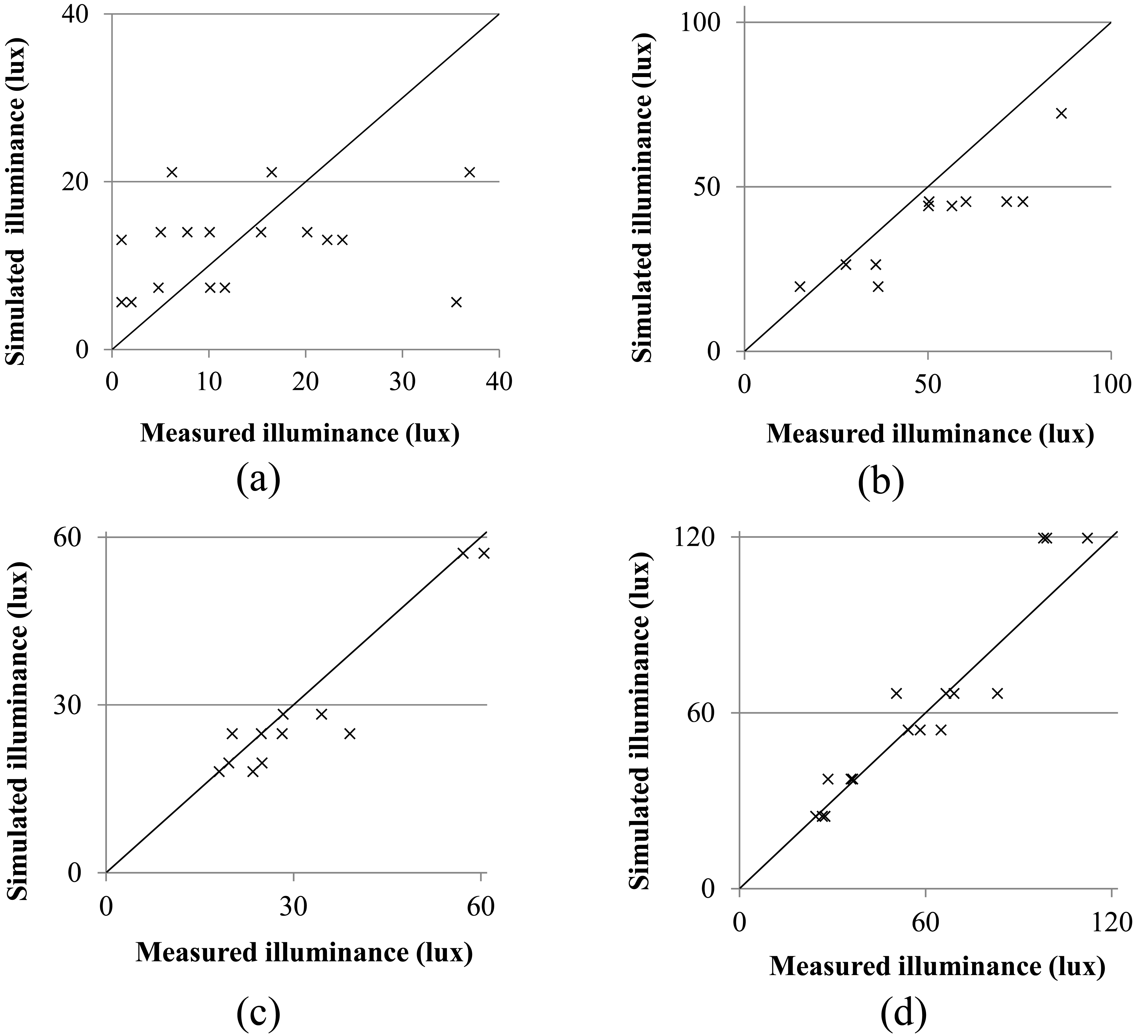
Fig. 4. Comparison of measured and simulated illuminance for (a) sensor v1, (b) v2, (c) s1, and (d) s2 with overcast conditions.

Figure 5

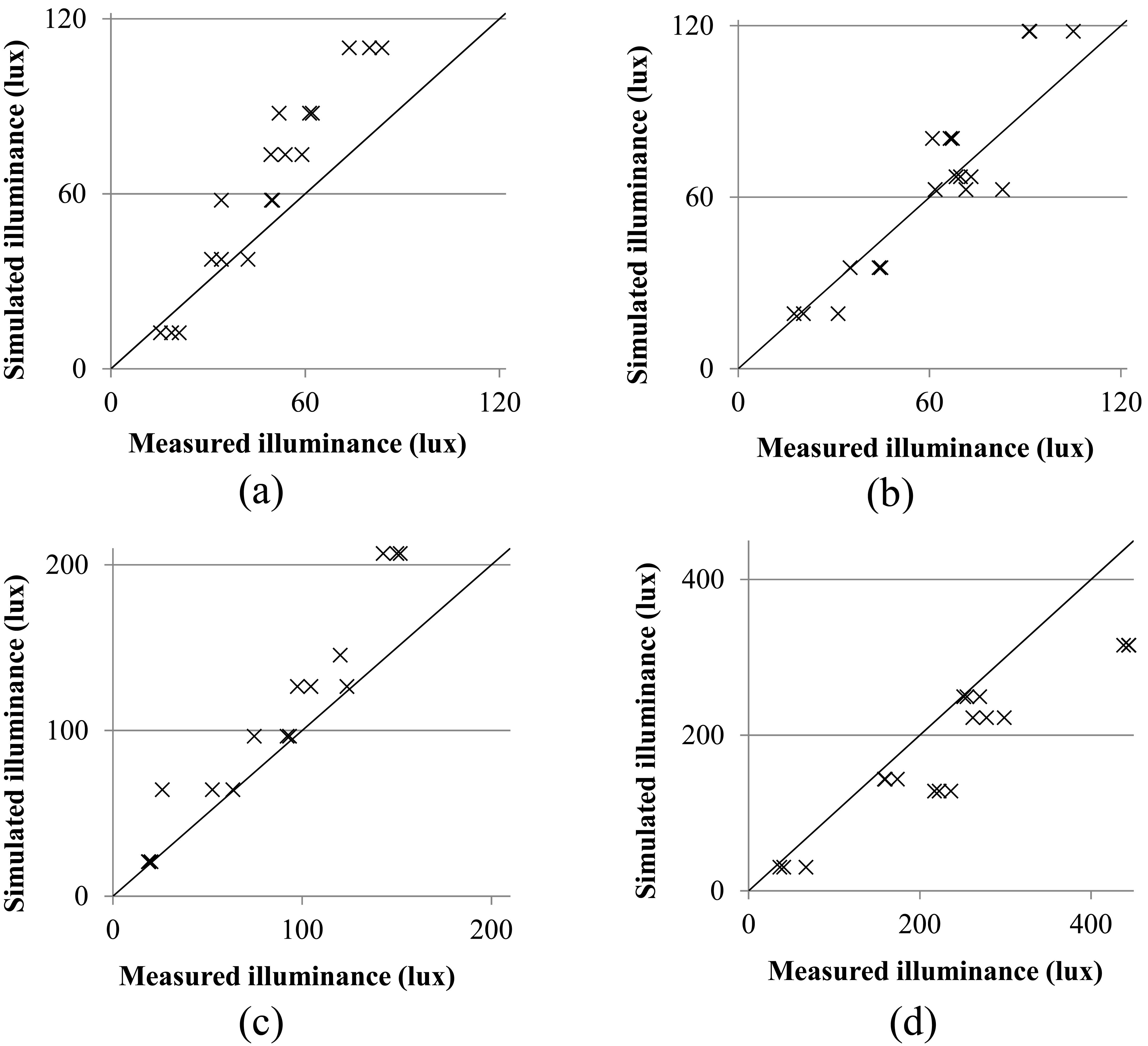
Fig. 5. Comparison of measured and simulated illuminance for (a) sensor v1, (b) v2, (c) s1, and (d) s2 with clear sky conditions and 3-28° solar altitudes.

In the case of clear skies, there is a trend to overestimate the values for higher illuminances in sensors v1 and s1 (Fig. 5(a) and (c), respectively). In the case of sensor s2, an inverse trend (progressive underestimation) is seen in Fig. 5(d). The trend for the simulations in sensor v2 (Fig. 5(b)) seems to approximately follow that of the measurements.

The AAD is displayed in Fig. 6. It confirms that the light levels are more stable for clear skies than for overcast skies and for sensors v2 and s2 (located below a light pipe) than for sensors v1 and s1 (located between two light pipes). It should be noted that this does not contradict the results in Table 7, which shows a lower discrepancy of the average values for overcast skies.

Figure 6

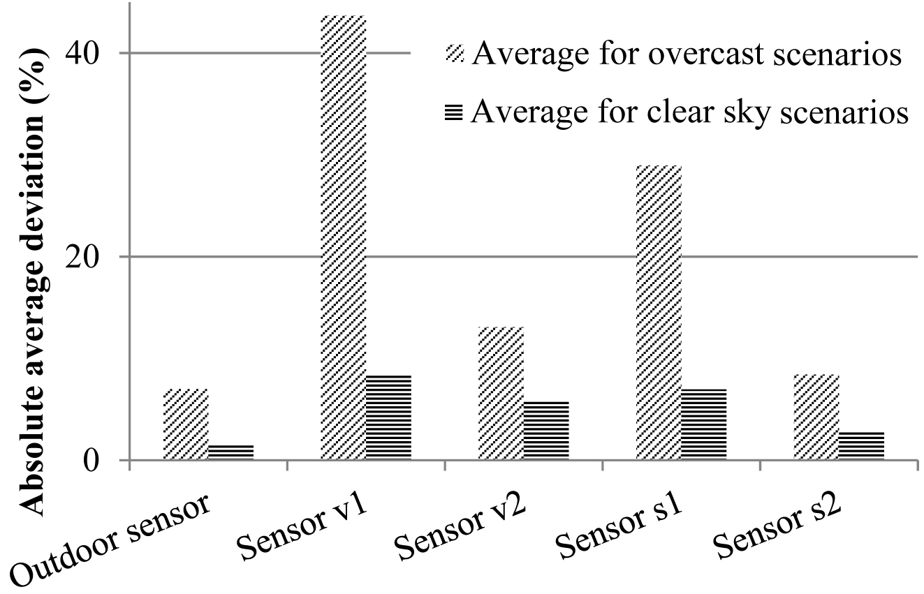
Absolute average deviation per sensor averaged for the 5 overcast times and the 4 of the 6 clear sky times (times CL2 and CL5 were excluded from the average).

Fig. 6. Absolute average deviation per sensor averaged for the 5 overcast times and the 4 of the 6 clear sky times (times CL2 and CL5 were excluded from the average).

3.2 Parametric study

The absolute illuminance value is usually given as incident illuminance at desk height or on the floor. However, in this case, it was considered more suitable to express it as luminous exitance from the diffuser because the distribution of light from the light pipe’s diffuser can vary largely from overcast to clear skies. For this reason, it was estimated that considering the light exiting from the diffuser and comparing it to the light falling on the collector was a more appropriate means to compare the performance of light pipes under overcast and clear skies.

Figure 7(a) shows the luminous exitance from the diffuser as a function of the solar elevation for both clear and overcast skies. The illuminance increases more rapidly for clear skies than for overcast skies.

Figure 7

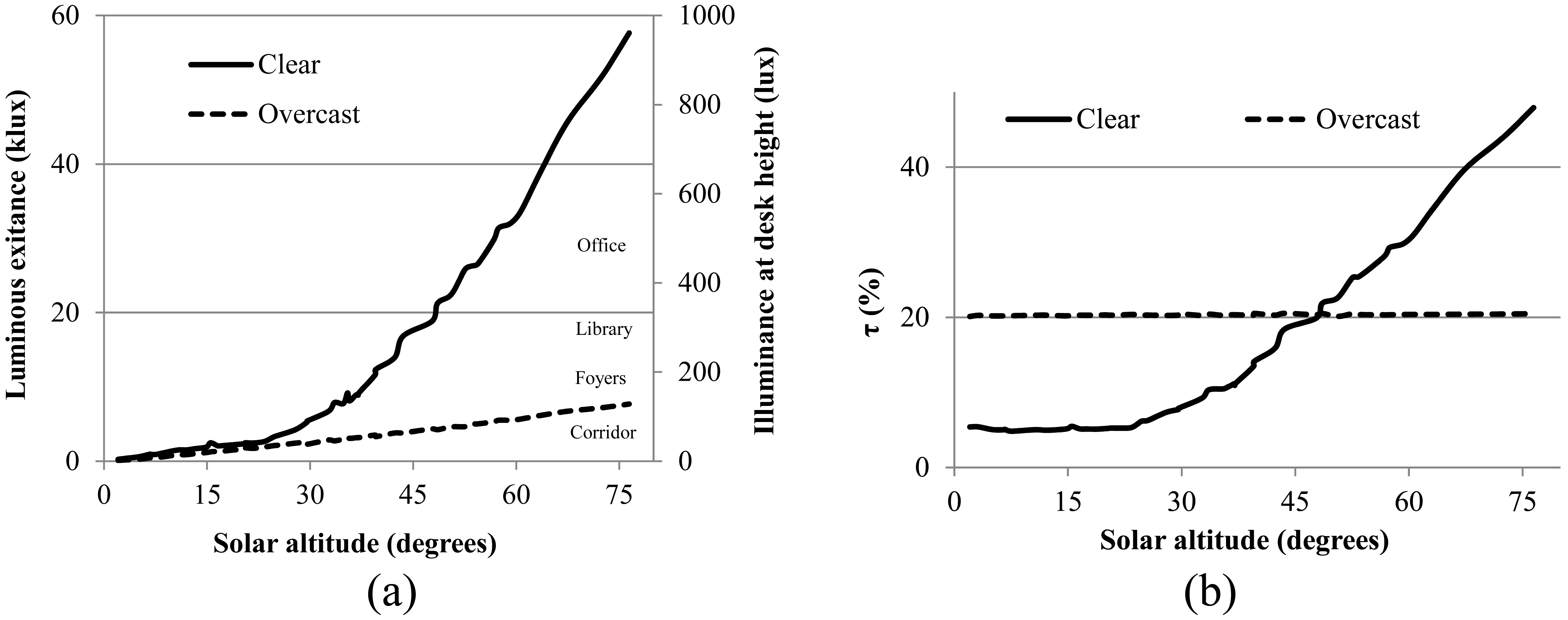
(a) Theoretical luminous exitance on the diffuser as a function of the solar altitude in the reference light pipe. (b) Theoretical luminous transmittance (τ) as a function of the solar altitude in the reference light pipe. Simulation was launched with TracePro® with a certain overestimation of sunlight in both diagrams.

Fig. 7. (a) Theoretical luminous exitance on the diffuser as a function of the solar altitude in the reference light pipe. (b) Theoretical luminous transmittance (τ) as a function of the solar altitude in the reference light pipe. Simulation was launched with TracePro^® with a certain overestimation of sunlight in both diagrams.

The forward raytracing method overestimated light output for higher solar altitudes with clear skies. Figure 8 was produced to put in perspective the results shown in Figure 7(a). It compares the trends of the simulated and measured values as the solar altitude is increased with clear sky conditions in sensor v2. The trend of the simulation results increases more rapidly compared to the trend obtained in the measurements. Sensor v2 was selected to be compared in this parametric study because it is also located below a light pipe with a flat collector.

Figure 8

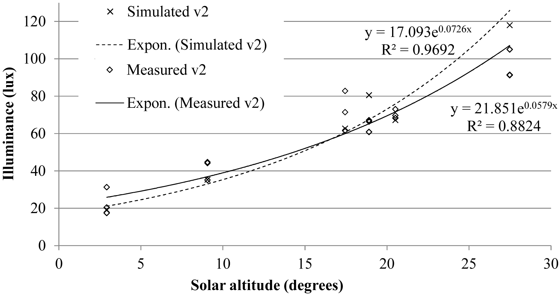
Fig. 8. Trend lines for measured and simulated illuminance on sensor v2 as a function of solar altitude.

Figure 7(b) shows the luminous transmittance in relation to the solar elevation both for clear sky and overcast conditions. As it can be seen, τ increases linearly from 35° of solar altitude for clear skies. On the other hand, τ is not affected by solar altitude for overcast skies. The impact of latitude on light pipe performance at different locations as well as luminous exitance on diffuser with different roof tilts in Lund at March and September 21st is shown in Fig. 9.

Figure 9

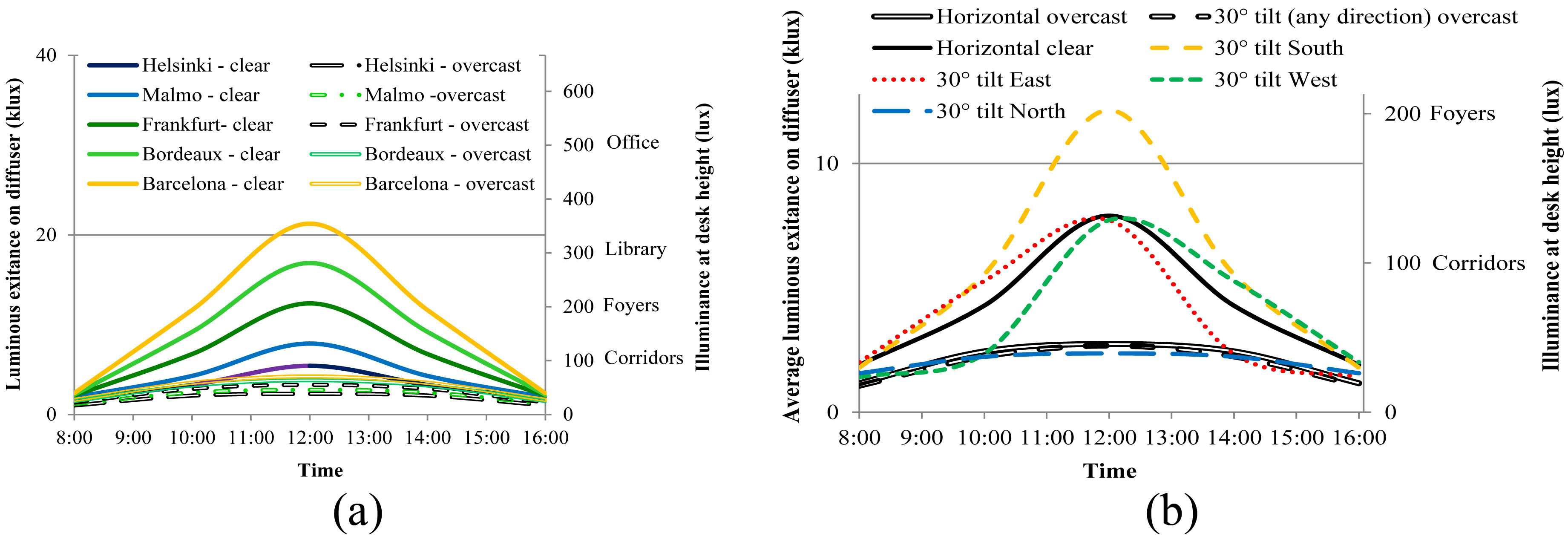
(a) Luminous exitance on the diffuser at different European cities on March and September 21st and (b) Luminous exitance on diffuser with different roof tilts on March and September 21st in Lund.

Fig. 9. (a) Luminous exitance on the diffuser at different European cities on March and September 21st and (b) Luminous exitance on diffuser with different roof tilts on March and September 21st in Lund.

4. Discussion

4.1 Variability of measurements

The variability of clear and overcast sky results require a separate discussion. The overcast skies illuminance levels and distribution strongly depend on the composition of the cloud layers, which makes the readings more variable and difficult to predict than in the case of clear skies. According Fig. 6, the illuminance variability is two to five times larger for overcast skies than for clear skies. These fluctuations between measurements are also illustrated by the wide distribution of points in Fig. 4. In spite of this large variability, the average of the measurements does follow the same trend as the simulated values. By using HDR images from the actual simulated sky [6], the uncertainty caused by the sky distribution could be avoided but this was not tested in the present study.

The sensor position in relation to the light pipe diffuser is shown in Fig. 6. The variability of daylight level as a function of sensor position is affected by sky type. With overcast skies, the low illuminance levels reaching the v1 and s1 sensors (5 to 30 lux) are operating close to their stated accuracy level. This could mean that sensor errors for low illuminance conditions would be larger. However, recorded data seems to have a linear response to increased illuminance [10].

In the case of clear skies, the difference between “v1 and s1” and “v2 and s2” sensors can be related to the shape of the light beam. Figure 10 shows a ring of light on the floor produced by sunlight transmitted through a light pipe. The size of this ring is very sensitive to variations in sun position, as shown in Fig. 11(a). Small inaccuracies in the model or in the simulation of the sun position could have caused a different ring pattern. This was estimated to be a leading cause of the higher light variability on “v1 and s1” sensors with clear skies. This demonstrates the importance of locating the sensors below a light pipe diffuser to reduce the variability in the illuminance readings.

Figure 10

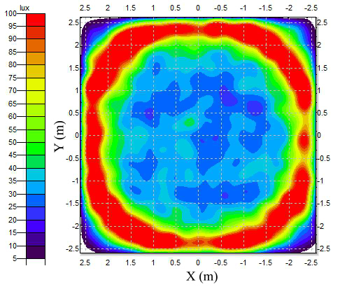
Fig. 10. Illuminance distribution on the floor by direct sunlight using the light pipe.

Figure 11

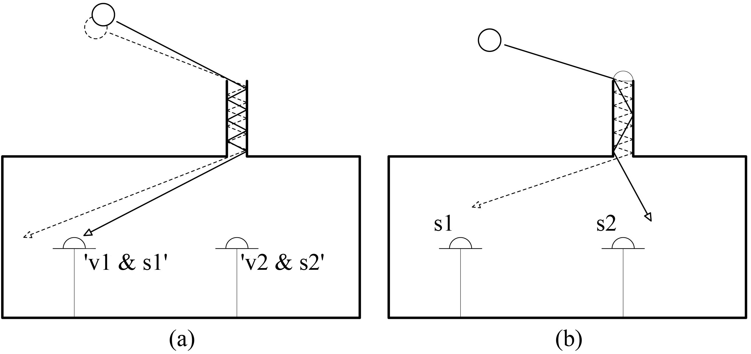
(a) Diagram showing how a small variation of the solar angle can have a significant impact in the light reaching (diffusor ring pattern) the sensor. (b) Diagram showing how the lack of the characterization of the dome collector light bending properties causes overestimation in “s2” and underestimation in “s1”.

Fig. 11. (a) Diagram showing how a small variation of the solar angle can have a significant impact in the light reaching (diffusor ring pattern) the sensor. (b) Diagram showing how the lack of the characterization of the dome collector light bending properties causes overestimation in “s2” and underestimation in “s1”.

4.2 Correspondence between measurement and simulation results

The discrepancy between simulated and measured values was lower for overcast than clear sky conditions for all sensors. With a total error of about ± 20%, this relative discrepancy can be considered as acceptable for early design stage predictions [18]. With overcast skies, the simulated values differed by less than 20% compared to the average of measurements in 85% of the cases and in 42% of the cases for clear skies.

Under clear skies, the error was increasing as illuminance, and solar altitude increased for three of the four sensors. The simulations in house 1 matches the measurements for one sensor (v2) and overestimates them for the other one (v1). In house 2, one sensor overestimates (s1) the measurements, and the other one underestimates them (s2).

In house 1, all the elements of the light pipes were correctly characterized including the BSDF of the diffuser, which was provided by the manufacturer. The overestimation of the illuminance values in sensor v1 was most probably an incorrect representation of sunlight. Sensor v1 was lit by sunlight while sensor v2 (valid simulation) was only lit by the skylight. Figure 12 shows how direct sunlight is shaded from the collector of light pipe three, located on the north pitch of the roof. This light pipe lights sensor v2. On the other hand, sensor v1 (overestimated trend) is located between light pipes one and two that receive sunlight. This leads to the conclusion that the direct sun contribution was overestimated and sky light was correctly simulated. The use of HDR images of the simulated skies could solve this problem according to [19].

Figure 12

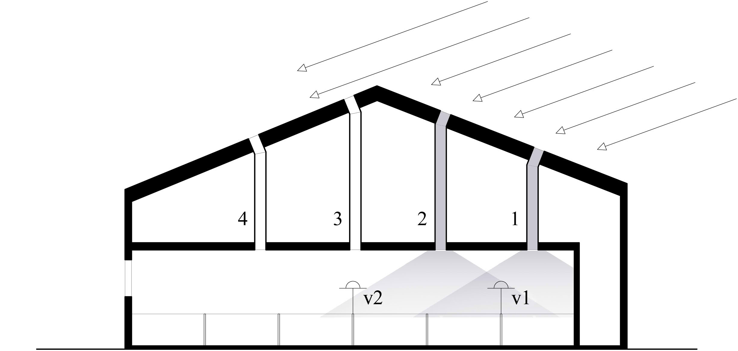
Fig. 12. Sensor v1 is reached by sunlight while sensor v2 is not illuminated by sunlight.

In house 2, the opposite trends (overestimation and underestimation) in the sensors can be explained by the absence of goniophotometric measurements for the dome collector of house 2. This element is an ORS that requires this type of information to take into consideration its light bending properties. Figure 11(b) illustrates how the sunrays are redirected into the pipe at lower angles reaching the area around “s1”. The simulated rays (dotted line) are not bent in the collector and reach the room at lower angles, producing an overestimation in “s2” and an underestimation in “s1”. Theoretically, the trends would have been similar to the one of sensor v2 in stable 1 (overestimation due to sunlight) if it had been possible to simulate the collector dome’s light bending properties by including its goniophotometric characterization.

The analyzed light pipes of house 2 show higher light output than the ones of house 1. This is due to many factors: higher light pipe reflectance, higher specular reflectance, higher transmittance in the collector and the diffuser, the innovative dome, etc. The large differences between sensors v2 and s2 are to a high extent caused by the fact that the house 2 collector was exposed to sunlight while the collector of house 1 was shaded by the roof ridge. It was also noted that the light redirecting properties of the house 2 dome collector results in a narrower light beam than in the case of the house 1 light pipes.

4.3 Parametric study

4.3.1 Solar altitude

The solar altitude is the parameter with the highest impact on the light output from the light pipes, especially for clear skies (Fig. 9). The results of this study show that the simulation method overestimated sunlight under clear skies as the solar altitude increased, which is also illustrated in Fig. 8, where the trend line of the measurements and that of the simulation values show a similar exponential growth. According to Fig. 7(b), the percentage of luminous transmittance that goes through the light pipe with overcast skies stays constant as the solar altitude is varied. This indicates that the slight increase in luminous exitance under overcast skies (Fig. 7(a)) is probably caused by the increase in GHI (factor 1 in Table 6). This is due to the fact that the illuminance distribution of overcast skies is constant for all sun positions.

The difference in light output from the light pipe between overcast and clear skies is confirmed by the illuminance measurements in the pig houses. The difference in light reaching sensor s2 in CL4 is 280% higher than in OC1, and only 8% higher for sensor v2. This demonstrates the significant effect of sunlight on light pipe’s output.

Solar altitude is linked to latitude and therefore light pipes are more effective when used in southern Europe than in Scandinavia for two reasons: solar altitude and sky clearness (direct sunlight occurs during around 2000 hours in southern Europe and only about 1000 hours in Scandinavia).

4.3.2 Aspect ratio

The aspect ratio determines the amount of light bounces in the pipe and can be manipulated by the designer. Increasing the aspect ratio from 0.1 to 0.06 led to an 11.5% increase in illuminance on the summer solstice at midday and 6% on the winter solstice at midday. However, the increase of luminous transmittance as a function of aspect ratio is not dependent on solar altitude for overcast skies. An equivalent increase in aspect ratio under overcast skies produced an increase of 4.5% in luminous transmittance.

4.3.3 Light pipe illuminance

The specular reflectance has a drastic effect on the luminous transmittance of the light pipe. In this case, a τ increase of about 1% to 3% can be observed for each additional percentage increase in reflectance – the highest increases corresponding to higher solar altitudes.

The light pipe’s luminous transmittance increased by 1.5% to 4% for each percentage increase that was transferred from diffuse to specular reflectance. This proves the importance of improving the pipe’s specular reflectance to obtain better light outputs from light pipes.

4.3.4 Roof tilt orientation

The impact of roof tilt on light pipe’s output is negligible at winter solstice with illuminance levels of 10 to 30 lux at desk height, which is below the reference value for corridors (100 lux) due to very low solar altitudes below 11°. A tilt of 30° to the south increased the peak of the illuminance curve at midday by 52% and 32% for March and June, respectively. If the roof tilt was 30° to the north, the illuminance peak was reduced by 71% and 40%. The effect of the tilts on the illuminance is highest around midday and decreases towards the morning and evening. With overcast skies, horizontal roofs are optimum for light pipes.

4.4 Improving light pipe simulation

Some recommendations to simulate light pipes using the forward raytracing method are stated below:

The specular and the diffuse reflectance of the pipes needs to be described with accuracy, since small inaccuracies can produce significant errors.
Goniophotometric properties of all the ORS in the light pipes need to be described by a detailed BSDF, especially for simulations with clear skies. This information should be provided by the manufacturers. The goniophotometric definition of the diffuser affects the distribution of the light output, while the goniophotometric definition of the collector also affects the luminous transmittance of the light pipe.
GHI can vary significantly with overcast skies. By simulating and measuring the outdoors GHI at the specific moment a factor can be obtained to weigh the results.

Another additional measure that can help to improve the accuracy of the results is the use of HDR images of the simulated skies instead of generic sky models. This method also allows the simulation of intermediate skies.

The illuminance values produced by light pipes fluctuate significantly over short periods, especially with overcast skies. Some measures that can be taken to limit this variability include:

Placing the sensors below the light pipe diffuser.
Considering several consecutive measurements.
Not considering very low illuminance values in the same order of magnitude as the sensor error margin.
Not considering dusk or dawn because light levels are very low and vary rapidly during these moments of the day.

5. Conclusions

In this study, a forward raytracing simulation method was evaluated for two light pipe systems, where the simulated light output results were compared to the illuminance measurements in two pig stables. In addition, a parametric study allowed assessing key design parameters of light pipe design.

Daylight was measured in two identical pig stables, fitted with four light pipes each, with three continuously measuring sensors in each stable and an outdoor sensor during 2013 and 2014. A forward raytracing tool, TracePro®, was used to predict the illuminance and parametric simulation.

The simulation results for overcast skies presented discrepancies between the simulated and average measurements below 30% in 100% of the cases. The discrepancies for clear skies were higher: below 30% discrepancy in 67% of the cases. With a total error of about ± 20%, which can be considered as acceptable for early design stage predictions, the simulated values with overcast skies differed by less than 20% compared to the average of measurements in 85% of the cases and in 42% of the cases for clear skies. The higher discrepancies with clear skies were due to the overestimation of sunlight and the absence of an advanced and detailed optical characterization of the dome collector surface for house 2 (Solatube^®).

To minimize inaccuracies in using forward raytracing, specular and diffuse reflectance of the pipes need to be described accurately and goniophotometric properties of all optical redirection system in the light pipes need to be described by an advanced and detailed optical characterization, especially for clear sky simulations. Since GHI can vary significantly with overcast skies, the use of HDR images of the simulated skies could improve results and allow the simulation of intermediate skies.

The parametric results showed that light pipes perform better during summer time, in sunny climates, at low to mid-latitudes with higher solar altitudes (south Europe) than during winter and in cloudy climates at high latitudes like Scandinavia. Methods to improve the luminous transmittance for low solar altitudes include: bending or tilting the pipe, increasing the aspect ratio, improving the pipe’s specular reflectance, tilting the collector to the south, or using optical redirection system in the collector.

Acknowledgements

The authors gratefully acknowledge the financial support from the Swedish Energy Agency (36459-1), Region Skåne Fund for Environmental Studies (M 080) and the Swedish Farmers Accident Insurance Fund (H132-0027-SLO). We also thank Mats Olsson and Thomas Nilsson for support in carrying out the experiments.

Contributions

N. Gentile performed the pig house measurements. A. Pacheco Diéguez’processed results wrote a manuscript outline and M-C Dubois contributed to the results analysis and the manuscript. H. von Wachenfelt conceived the study and wrote the manuscript with input from all the authors. All the authors discussed the results.

References

T. Whitted, An improved illumination model for shaded display, Commun. ACM 23 (1980) 343–349. http://dx.doi.org/10.1145/358876.358882
T. Kolås, Performance of Daylight Redirecting Venetial Blinds for Sidelighted Spaces at High Latitudes, Performance analysed by forward raytracing simulations with the software TracePro, Thesis for the degree of Philosophiae Doctor, Trondheim, Norwegian University of Science and Technology, Faculty of Architecture and Fine Art, Department of Architectural Design, Form and Colour, 2013.
S. Dutton and L. Shao, Raytracing simulation for predicting light pipe transmittance, International Journal of Low-Carbon Technologies 2 (2007) 339–358. http://dx.doi.org/10.1093/ijlct/2.4.339
C. Kohler, NFRC presentation, from Initial summary of round robin tvis measurements for tubular daylighting devices (TDD), Available online: http://www.nfrc.org/documents/ComplexProductVTpresentation_April2010ss.pdf (accessed on 21 January 2014).
A. Farrel, B. Norton, and D. Kennedy, Lightpipe daylight simulation modeling using Radiance backward and forward ray-tracing methods: A comparison with monitored data for commercial light pipes in Ireland, in: Third International Radiance Workshop, École d’ingénieurs et d’architectes de Fribourg, 2004, Switzerland.
M. Inanici, Evaluation of High Dynamic Range Image-Based Sky Models in Lighting Simulation, LEUKOS: The Journal of the Illuminating Engineering Society of North America, 7 (2010) 69–84. http://dx.doi.org/10.1582/LEUKOS.2010.07.02001
J. Mardaljevic, L. Heschong, and E. Lee, Daylight metrics and energy savings, Lighting Research and Technology 41 (2009) 261–283. http://dx.doi.org/10.1177/1477153509339703
SJV, Swedish Animal Welfare Agency, Swedish Board of Agriculture, SJVFS 2014:31 L100, in Swedish, Jordbruksverket, 2014.
CEC, Commission Directive 2001/93/EC of 9 November 2001 amending Directive 91/630/EEC: Laying down minimum standards for the protection of pigs, Commission of the European Communities, Brussels, Belgium, 2001.
H. von Wachenfelt, V. Vakouli, A. Pacheco Diéguez’, N. Gentile, M-C. Dubois, and K-H. Jeppsson, Lighting energy saving with light pipe in farm animal production, Journal of Daylighting 2 (2015) 21–31. http://dx.doi.org/10.15627/jd.2015.5
Lambda Research Corporation, TracePro® User Manual, Release 7.4, 2014.
TracePro®, Available online: http://www.lambdares.com/tracepro (accessed on 16 March 2014).
IEA, International Energy Agency, Monitoring Procedures for the Assessment of Daylighting Performance of Buildings, A Report of IEA SHC Task 21 / ECBCS Annex 29, 2001.
K-H. Jeppsson, D. Nilsson, H. von Wachenfelt, and T. Hörndahl, Lighting design in animal buildings with DiaLux and a quantitative assessment of lighting environment on pasture vs indoors for cattle, in Swedish, LTJ-report 2013:34, Alnarp, 2014.
N. Igawa, Y. Koga, T. Matsuzawa, and H. Nakamura, Models of sky radiance distribution and sky luminance distribution, Solar Energy 77 (2004) 137–157. http://dx.doi.org/10.1016/j.solener.2004.04.016
J. Murdoch, Illumination Engineering – from Edison´s lamp to the laser, Macmillan Pub. Co, 1985.
L. Kómar and S. Darula, Determination of the light tube efficiency for selected overcast sky types, Solar Energy 86 (2012) 157–163. http://dx.doi.org/10.1016/j.solener.2011.09.023
D. H.W. Li, E. K.W. Tsang, K.L. Cheung, and C.O. Tam, An analysis of light-pipe system via full-scale measurements, Applied Energy 87 (2010) 799–805. http://dx.doi.org/10.1016/j.apenergy.2009.09.008
J. Stumpfel, C. Tchou, A. Jones, T. Hawkins, A. Wenger, and P. Debevec, Direct HDR capture of the sun and sky, in: 3rd International Conference on Computer graphics, virtual reality, visualisation and interaction in Africa, 2004, 145–149.

Get PDF (2.82 MB)

SHARE ON