Phasor Method to Estimate Illuminances Due to Parallel Arrays of Light Sources

^a Building Physics Research Group, Faculty of Industrial Technology, Institut Teknologi Bandung, Jl. Ganesha 10, Labtek VI, Bandung 40132, Indonesia
^b Engineering Physics Doctorate Program, Faculty of Industrial Technology Institut Teknologi Bandung, Jl. Ganesha 10, Labtek VI, Bandung 40132, Indonesia
^c Architecture Program, Faculty of Engineering, Universitas Malikussaleh, Jl. Cot Teungku Nie, Aceh Utara 24355, Indonesia

* Corresponding author.
armanto@tf.itb.ac.id (R. A. Mangkuto)
atthaillah@unimal.ac.id (Atthaillah)

History: Received 2 October 2020 | Revised 4 November 2020 | Accepted 16 November 2020 | Published online 30 November 2020

Citation: Rizki A. Mangkuto, Atthaillah, Phasor Method to Estimate Illuminances Due to Parallel Arrays of Light Sources, Journal of Daylighting 7 (2020) 246-257. https://dx.doi.org/10.15627/jd.2020.21

Figures and tables

Figure 1
Figure 2
Figure 3
Figure 4
Figure 5
Figure 6
Figure 7
Figure 8
Table 1
Table 2
Table 3
Table 4
Table 5
Figure 9
Table 6
Figure 10
Figure 11
Figure 12
Figure 13

Abstract

Direct horizontal illuminance along a calculation row due to two parallel arrays of large numbers of identical light sources behaves like a periodic signal with a sinusoidal pattern, which contains useful information for design purpose. This study aims to describe, verify, and discuss the theoretical concept on the superposition of direct horizontal illuminance from both arrays in such configurations, and how to extract the information using the phasor method. Four different approaches are proposed to estimate the total direct horizontal illuminance E_T(x) and to verify the concept. Sensitivity analysis is also conducted to observe the influence of each input variable to the resulting E_T(x) pattern. The differences between obtained values using the four approaches are found very small, so that the proposed concept is verified. Based on the sensitivity analysis, the luminous intensity distribution of the sources significantly affects the illuminance fluctuation; whereas the impact of lateral position of the calculation row and the spatial phase difference are inconsistent. Overall, the advantage of using phasor method has been demonstrated for this purpose, which is expected to help in understanding the superposition phenomenon of sinusoidal pattern of illuminance, and in achieving the desired spatial contrast.

Keywords

Phasor method, Horizontal illuminance, Sinusoidal pattern, Parallel array

Nomenclature

BZ	British zonal
E_P	Horizontal illuminance on a point [lx]
E(x)	Horizontal illuminance along the calculation row [lx]
E_med(x)	Median horizontal illuminance along the calculation row [lx]
E_min(x)	Minimum horizontal illuminance along the calculation row [lx]
E_max(x)	Maximum horizontal illuminance along the calculation row [lx]
I₀	Maximum luminous intensity of the source, at γ = 0 [cd]
k	Wavenumber [m^–1]
LID	Luminous intensity distribution
n	Power coefficient in the cosine-like LID model
x	Longitudinal position along the calculation row [m]
y	Lateral position of the second array with respect to the first array [m]
y_P	Lateral position of the calculation row with respect to the first array [m]
γ	Zenith angle of luminous intensity, relative to the source’s normal [rad]
z	Mounting height of the source [m]
β’	Standardised regression coefficient [-]
ΔE	Horizontal illuminance fluctuation [lx]
δ	Spatial phase difference, longitudinal distance between arrays [m]
ϕ	Angular phase difference [rad]
ξ(x)	Complex notation of horizontal illuminance along the calculation row [lx]
λ	Spatial wavelength, distance between adjacent sources [m]

1. Introduction

Calculation of illuminance on the workplane or reference plane is one of the most important tasks to perform in lighting engineering and design. Starting from the prominent work of Lambert in the 18^th century [1], most of the procedures for illuminance calculation have been well-established in the last century [2,3] and thus have become standard knowledge for lighting engineers and designers.

The advance of computational lighting modelling and simulation in the past decade [4-6] also greatly reduces the need for manually performing routine illuminance calculation, and so contributes in providing better and more accurate design recommendations. Nevertheless, it is important for any lighting engineers and designers to understand the underlying principles used in the calculation processes, to minimise the risk of having unreliable results [7]. The knowledge of the underlying principles shall enable engineers or designers to write their own (computer) programs or algorithms whenever necessary; and would be a valuable material for education purpose [7-9].

Despite seeming to be well-understood, one of the topics that tends to be overlooked is the the horizontal illuminance (E_P) calculation due to parallel arrays of identical light sources mounted at an equidistant interval, forming a periodic spatial pattern. An example would be the configuration of pendant luminaires in a library (Fig. 1), which consists of two parallel rows (or arrays) of luminaires. Since the mounting height and the distance between adjacent luminaires at the same array are typically constant, the direct E_P values at a given calculation row parallel to the arrays also follows a periodic spatial pattern. For typical interior luminaires, the periodic pattern is expected to be a sinusoidal one, provided the number of luminaires in each array is large enough.

Figure 1

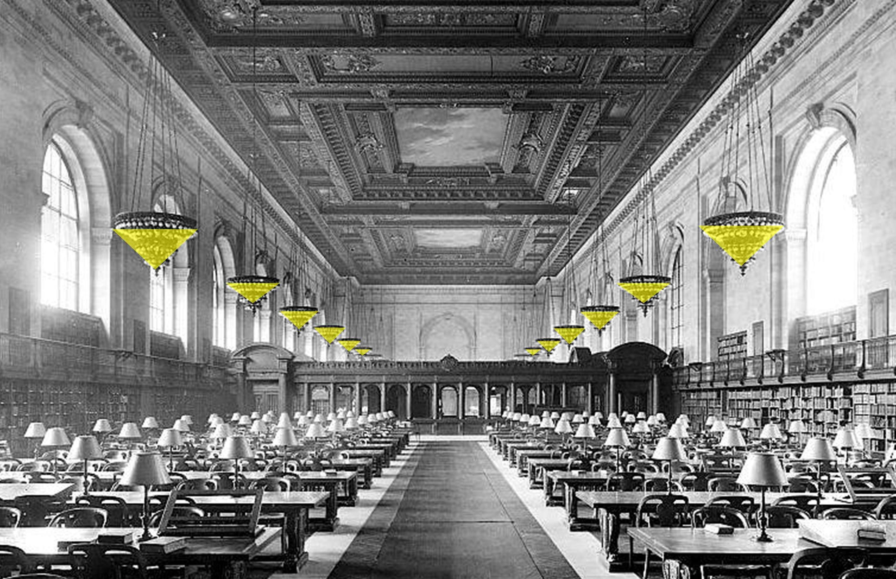
Illustration of two parallel arrays of luminaires (highlighted in yellow) with a periodic pattern. (adapted from public domain image: Main Reading Room of the New York City Public Library on 5th Avenue, ca. 1910–1920).

Fig. 1. Illustration of two parallel arrays of luminaires (highlighted in yellow) with a periodic pattern. (adapted from public domain image: Main Reading Room of the New York City Public Library on 5th Avenue, ca. 1910–1920).

The direct E_P along the calculation row due to a single array of luminaires therefore behaves like a periodic signal, stationary in time (assuming the sources are constantly turned on) but varying in one-dimensional space of interest. Combining both arrays of luminaires together shall yield another sinusoidal pattern, which is basically the superposition of two sinusoidal signals. The pattern contains several important information, such as the values and positions of maximum and minimum illuminances along the calculation row, which can be useful for design purpose.

The example can be also extended, for instance, in the lighting arrangement above the audience seats in theatres. To a certain extent, one can also think on arrays of windows or clerestories on both long sides of a corridor under the CIE overcast sky. All those scenarios shall reveal a sinusoidal pattern of E_P along a calculation row parallel to the sources. When the calculation row is located for instance on a diffuse floor, the resulting illuminance pattern may also be correlated with luminance difference and spatial contrast, which is considered an integral part of the architectural features of the space [10,11]. Spatial contrast is found to be an important factor in indoor (e.g. [11-15]) and outdoor spaces (e.g. [16-19]). In a typical indoor office setting, for instance, it is known that luminance diversity and non-uniform lighting distribution may be positively correlated with and the occupants’ impression of excitement and preference [20,21], although a space with too excessive luminous variability may be perceived as uncomfortable [22].

The concept of spatial brightness and perceived adequacy of illumination (PAI) in lighting design has also been promoted in the past decade [12,23,24]. The existence of spatial patterns is also typically indicated with luminance contrast, in the case of indoor spaces [11,14]; and mean, minimum, and maximum illuminances in the case of outdoor spaces (or any space with relatively low reflections from the environment), particularly streets or roads [17-19].

The information contained in the sinusoidal pattern is however seldom discussed in literatures and standards. This study therefore aims to describe and discuss the theoretical concept on the superposition of direct E_P from both sources’ arrays in such configurations, and to verify it with some worked examples. The article is structured as follows: Section 2 provides the theoretical concept of the relevant calculations for obtaining the direct E_Pdue to two parallel, periodic arrays of identical sources. Section 3 describes the methods applied in verifying the proposed concept, followed with sensitivity analysis on the input variables. Sections 4 and 5 provides the results and discussion, whereas Section 6 concludes the article.

2. Concept

Consider an array comprising a large number of identical light sources, i.e. those with identical luminous flux and luminous intensity distribution (LID), mounted at a constant height z above the reference plane. The LID of the sources is assumed to be cosine-like, i.e. closely follows that of BZ1 or up to BZ5 type in the British Zonal (BZ) classification system [25,28]. Adjacent sources are separated by a constant distance λ, as illustrated in Figs. 2(a), 3(a), and 4(a). Suppose there exists a row of calculation points, parallel with the sources array at a lateral distance y.

Figure 2

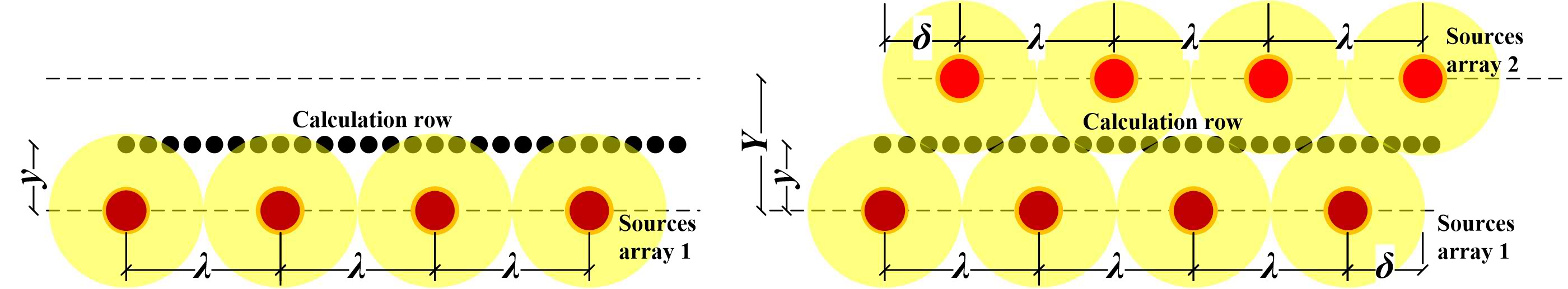
Plan view of (a) a periodic array and (b) two parallel, periodic arrays of identical light sources with a constant distance λ. The black dots in the middle represent the row of calculation points for horizontal illuminance.

Fig. 2. Plan view of (a) a periodic array and (b) two parallel, periodic arrays of identical light sources with a constant distance λ. The black dots in the middle represent the row of calculation points for horizontal illuminance.

Figure 3

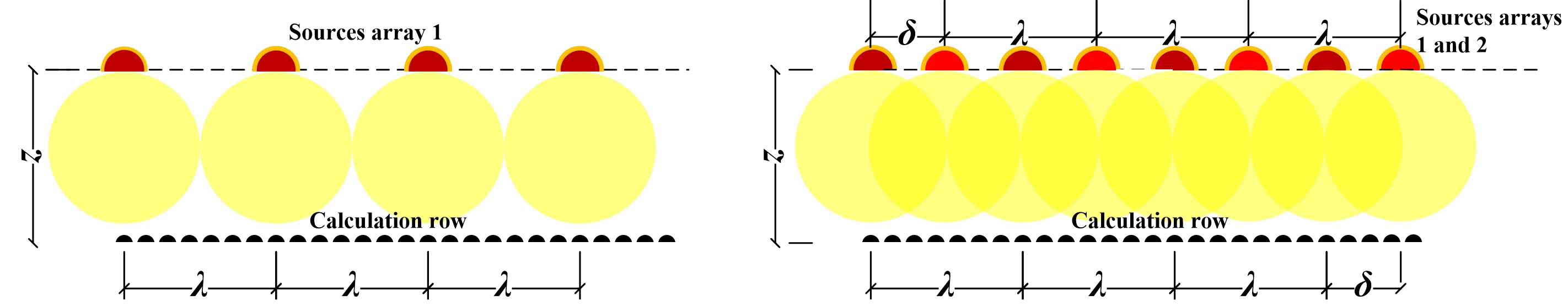
Fig. 3. Elevation view of (a) a periodic array and (b) two parallel, periodic arrays of identical light sources with a constant interval λ, as per Fig. 2.

Figure 4

Fig. 4. Perspective view of (a) a periodic array and (b) two parallel, periodic arrays of identical light sources with a constant interval λ, as per Fig. 2.

The direct E_P values on the calculation points are expected to vary according to a sinusoidal pattern, as illustrated in Fig. 5. One can thus observe the maximum, median, and minimum E_P values (E_max, E_med, E_min) along the calculation row. Since the LID of the sources is assumed to follow BZ1 or up to BZ5 type, the source’s luminous intensity at any zenith angle γ reads:

\[ I_\gamma=\left\{\begin{matrix}I_0\cos^n{\gamma},\mathrm{\ \ }\ 0\le\gamma\le\pi\mathrm{/2}\ \\0,\ \ \ \ \ \ \ \ \ \ \ \ \ \ \ \ \ \pi\mathrm{/2}<\gamma\le\pi\\\end{matrix}\right. \]

where I₀ is the maximum luminous intensity at γ = 0; while n = 4, 3, 2, 1.5, and 1 respectively for BZ1, BZ2, BZ3, BZ4, and BZ5. Therefore, E_max will be achieved at position that is the nearest to an individual source (e.g. directly beneath it), while E_min will be achieved at position that is the farthest to any individual source (e.g. midway between two adjacent sources).

From Fig. 5, it is clear that the median (also the mean) of the E_P values is:

\[ E_{med}=\frac{E_{\mathrm{max}}+E_{min}}{2}, \]

whereas one can define E_o as the difference between E_max and E_med, which is equal to the difference between E_med and E_min, which also reads:

\[ E_o=\frac{E_{\mathrm{max}}-E_{min}}{2} \]

Figure 5

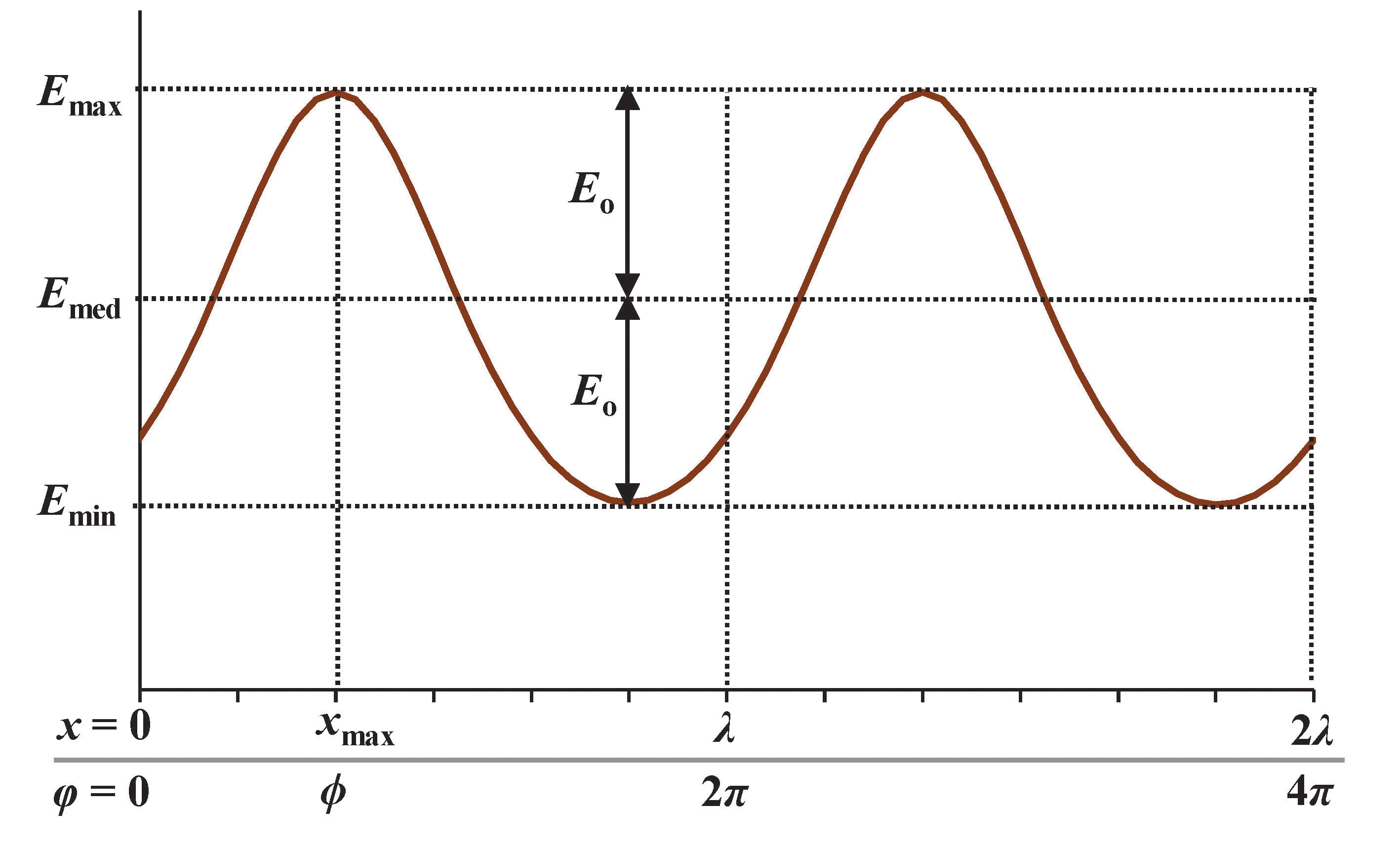
Fig. 5. Sinusoidal pattern of direct horizontal illuminance due to a periodic array of identical sources.

The direct E_P values at any position x along the calculation row (E(x)) can therefore be described in the standard cosine form in Eq. (4) as follows:

\[ E(x)=E_o\cos{(}kx+\phi)+E_{\mathrm{med}} \]

where k is the wavenumber, equal to 2π/λ; and ϕ is the phase difference relative to the origin as shown in Fig. 5. It is common to say that according to the illustration of Fig. 5, ϕ is negative (i.e. the signal is lagging behind). The distance x_max (measured from x = 0) at which E_max occurs is thus:

\[ x_{max}=-\frac{\phi}{2\pi}\lambda=-\frac{\phi}{k} \]

Consider now another array comprising a large number of identical sources mounted at a constant height above the reference plane, also with a constant interval λ, but with a spatial phase difference δ. Suppose this array is located parallel with the first one, at a lateral distance Y, as shown in Figs. 2(b), 3(b), and 4(b). The mounting height of the sources in the second array is not necessarily the same with those in the first array (z), but it is practical and realistic to assume they are the same. If the contribution from each array is now measured individually, one can thus write:

\[ {E_1(x)=E_{\mathrm{o,}1}\cos{(}kx+\phi_1)+E_{\mathrm{med,1}}\mathrm{\ ,}\ \atop E_2(x)=E_{\mathrm{o,}2}\cos{(}kx+\phi_2)+E_{\mathrm{med,2}}\mathrm{\ ,}\ } \]

where E₁(x) and E₂(x) are respectively the direct horizontal illuminances at any position x along the calculation row due to the first and the second array. Notice that both arrays have the same wavenumber k, since the interval between adjacent sources in both arrays is constant.

Suppose that the contribution from both arrays are to be measured altogether. The resulting direct horizontal illuminance E_T(x) is thus the addition, or superposition, of E₁(x) and E₂(x). In the case where E_o,1 = E_o,2, i.e. when the lateral distances between the calculation row and both sources arrays are the same, the E₁(x) and E₂(x) can be simply added using trigonometric identities. Otherwise, it is easier to work the superposition using the phasor method, which is a routine technique in dealing with signal or wave interference.

In this case, the cosine terms in E₁(x) and E₂(x) shall be described as the real (Re) parts of the complex notations ξ₁(x) and ξ₂(x), which read:

\[ \xi_1(x)=E_{\mathrm{o,}1}[\cos{(}kx+\phi_1)+j\sin{(}kx+\phi_1)]=Eo,1ej(kx+ϕ1)=Eo,1ejkxeϕ1 , \atop \xi_2(x)=E_{\mathrm{o,}2}[\cos{(}kx+\phi_2)+j\sin{(}kx+\phi_2)]=Eo,2ej(kx+ϕ2)=Eo,2ejkxeϕ2 , \]

where j = √–1.

Since k is constant for both signals, the sum of both complex notations, ξ_T(x), reads:

\[ {\xi_T(x)=\xi_1(x)+\xi_2(x)=e^{jkx}(E_{\mathrm{o,}1}e^{j\phi_1}+E_{\mathrm{o,}2}e^{j\phi_2})\atop=e^{jkx}(E_{\mathrm{o,}T}e^{j\phi_T})\ =\ E_{\mathrm{o,}T}e^{j(kx+\phi_T)}\ .} \]

The variables E_o,T and ϕ_T can be determined using the phasor diagram as illustrated in Fig. 6. One can thus write:

\[ E_{o,T}=\sqrt{(E_{o,1}\cos{\phi_1}+E_{o,2}\cos{\phi_2})^2+(E_{o,1}\sin{\phi_1}+E_{o,2}\sin{\phi_2})^2} \]

\[ \phi_T=\arctan{\frac{E_{o,1}\sin{\phi_1}+E_{o,2}\sin{\phi_2}}{E_{o,1}\cos{\phi_1}+E_{o,2}\cos{\phi_2}}} \]

\[ E_T(x)=Re{{}\xi_T(x)}+E_{\mathrm{med,1}}+E_{\mathrm{med,2}}=E_{\mathrm{o,}T}\cos{(}kx+\phi_T)+E_{\mathrm{med,1}}+E_{\mathrm{med,2}}. \]

Figure 6

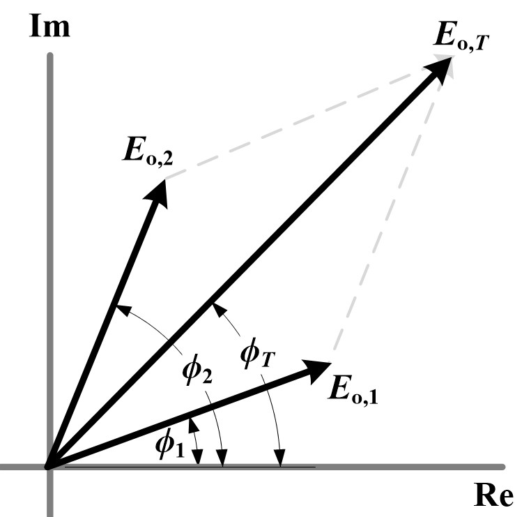
Fig. 6. Phasor diagram representing superposition of direct horizontal illuminance due to two parallel, periodic arrays of identical sources.

From Equation (11), the maximum, median, and minimum values of E_T(x) can therefore be determined respectively as follows:

\[ E_{max,{T}}=E_{\mathrm{o,}T}+E_{\mathrm{med,1}}+E_{\mathrm{med,2}}, \]

\[ E_{\mathrm{med},T}=E_{\mathrm{med,1}}+E_{\mathrm{med,2}}, \]

\[ E_{min,{T}}=-E_{\mathrm{o,}T}+E_{\mathrm{med,1}}+E_{\mathrm{med,2}}, \]

Having presented the concept, given a configuration of two parallel arrays of identical sources as previously described, one can estimate the E_T(x), by first calculating E₁(x) and E₂(x) at several discrete points along the calculation row (Fig. 7), followed by applying the phasor addition. The addition can be performed according to one of the following step-by-step approaches:

Figure 7

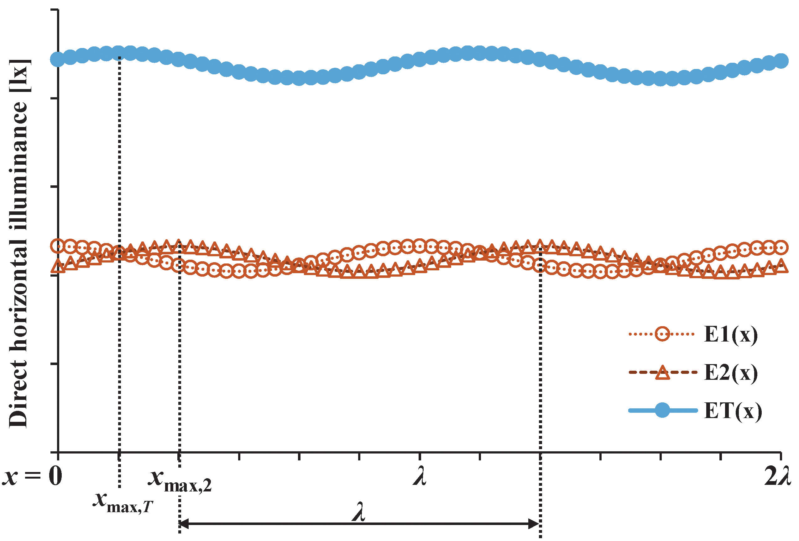
Illustration of discrete E1(x), E2(x), and ET(x) data along the calculation row.

Fig. 7. Illustration of discrete E₁(x), E₂(x), and E_T(x) data along the calculation row.

Approach 1 (phasor addition from regression model of discrete individual illuminance data):
Perform curve fitting using sinusoidal regression on the discrete E₁(x) and E₂(x) data. For both datasets, define the wavenumber k = 2π/λ, where λ is constant for both arrays of sources. Ensure that the coefficient of determination (R²) for both sinusoidal models are very close to 1.
Observe E_o,1, ϕ₁, E_med,1, E_o,2, ϕ₂, and E_med,2 values from the obtained models.
Add both models of E₁(x) and E₂(x) using the phasor method as per Equations (9) until (11), to obtain E_o,T, ϕ_T, and E_med,T.
Approach 2 (phasor addition from observation of discrete individual illuminance data):
Observe E_min, E_max, and x_max from the discrete E₁(x) and E₂(x) data.
Calculate E_o and E_med based on E_min and E_max for each dataset using Equation (3).
Calculate k = 2π/λ.
Calculate ϕ = –kx_max for each dataset using Equation (5).
Add both models of E₁(x) and E₂(x) using the phasor method as per Equations (9) until (11), to obtain E_o,T, ϕ_T, and E_med,T.

Results from both approaches shall be verifiable by directly observing the addition of E₁(x) and E₂(x) for each discrete point, thus giving discrete E_T(x) data as illustrated in Fig. 7, without applying the phasor addition. In turn, one of the following step-by-step approaches can be performed:

Approach 3 (regression model from observation of discrete total illuminance data):
Perform curve fitting using sinusoidal regression on the discrete E_T(x). Also define the wavenumber k = 2π/λ and ensure that R² à
Observe E_o,T, ϕ_T, and E_med,T values from the obtained models.
Approach 4 (observation of discrete total illuminance data):
Observe E_min,T, E_max,T, and x_max,T from the discrete E_T(x) data.
Calculate E_o,T and E_med,T based on E_min,T and E_max,T for each dataset using Equation (3).
Calculate k = 2π/λ.
Calculate ϕ_T = –kx_max,T for each dataset using Equation (5).

Based on the obtained coefficients in Approach 1 until 3, the E_min,T, E_max,T, E_med,T, and x_max,T can be estimated. The corresponding values obtained in all approaches are expected to be close to each other, provided the sinusoidal pattern is achieved. It should be noted that only a hypothetical configuration is described here, which are relevant to explain the theoretical concept of phasor addition in direct horizontal illuminance calculation. The function of the space is irrelevant in this part, because the concept is meant to be general, and thus is not affected by the absolute values of the horizontal illuminance. Material reflectance is assumed zero for all surfaces, because only direct horizontal illuminance is considered throughout the study. Dimensions are provided conceptually (with symbols) in Figs. 2-4, again because this section only provides the general concept, which is not affected by the absolute values of space dimensions. To further illustrate and test the concept, several examples are given in Section 3.

3. Methods

3.1 Verification

To give an illustration of the proposed concept in Section 2, consider the configuration of two parallel arrays of identical sources in Fig. 8. The distance between arrays (Y), the distance between adjacent sources (λ), and the mounting height (z) are set constant as 3 m. Each array consists of 14 identical downlight sources, each of having LID according to either BZ1 or BZ5 type, with the maximum luminous intensity of 1800 cd (i.e. yielding E = 200 lx at a point 3 m directly beneath the source’s centre). The observed space in Fig. 8 can be thought as a large reading hall in libraries (as in Fig. 1), provided a nighttime situation and a relatively low or negligible mean room surface reflectance. The specified maximum luminous intensity and the corresponding direct horizontal illuminance can thus be attributed to the chosen function.

Figure 8

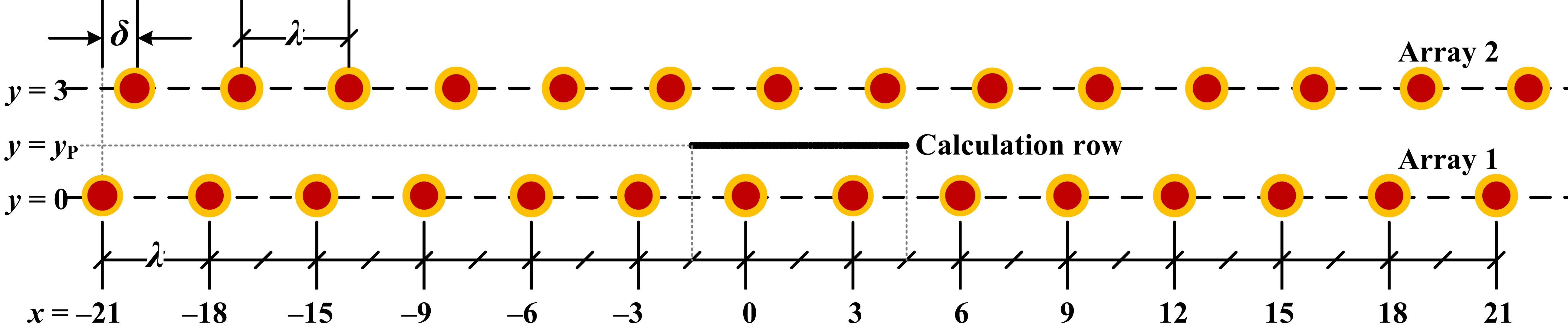
Fig. 8. Plan view of the tested configuration; units in meter.

There are 60 calculation points with an interval of 0.1 m along the calculation row, located at x = –1.5 until 4.5 m, according to the plan view in Fig. 8. The calculation row is at lateral distance y = y_P; where y_P = 0, 0.5, 1.0, or 1.5 m. The spatial phase difference δ between both arrays is defined as 0, 0.5, 1.0, or 1.5 m, all shifted towards the right-hand side of the first array. Table 1 lists all variables considered (LID, y_P, and δ) in the test. All combinations are considered, except the ones with y_P = δ = 1.5 m, because E₁(x) and E₂(x) will cancel each other out with respect to E_med, so that the resulting E_T(x) curves will be entirely flat and thus do not behave like sinusoidal signals. Therefore, in total there are 30 (= 2×4×4 – 2) combinations.

Table 1

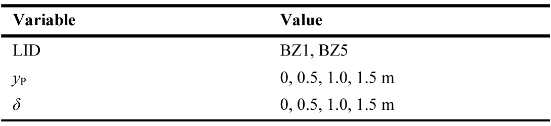
Table 1. List of all variables considered in the test.

While the length of the calculation row is only 6 m, it is necessary to introduce as many as 14 sources in each array to ensure the sinusoidal pattern is conserved in the calculation row. If there are too few sources in each array, the resulting E₂(x) due to shifted sources in the second array will be asymmetrical, because the calculation points on the left-hand side will see less contribution from the sources compared to the right-hand side.

The direct E_P at the i-th calculation point (E_P,i) due to an individual source S_i can be simply determined using the formula of point light source as follows:

\[ E_{P,i}=\frac{I_\gamma}{r_i^2}\cos{\alpha}=\frac{I_\gamma}{r_i^2}\frac{z}{r_i}=\frac{I_\gamma}{r_i^3}\cdot\ z. \]

where α is the angle between the line of sight and the normal of the calculation point; r_i is the distance between S_i and the calculation point. In this case, α = γ since the source’s and receiver’s normal are parallel. Substituting Equation (1) to (15), for 0 ≤ γ ≤ π/2, one can write:

\[ E_{P,i}=\frac{I_0}{r_i^3}\left(\cos{\gamma}\right)^n\cdot\ z=\frac{I_0}{r_i^3}\left(\frac{z}{r_i}\right)^n\cdot\ z=\frac{I_0z^{n+1}}{r_i^{n+3}}. \]

The total direct E_P at the i-th calculation point (E(x)) due to N number of sources is thus simply the sum of E_P,i from each source.

\[ E(x)=\sum_{i=1}^{N}E_{P,i}. \]

After performing routine calculations to obtain E(x) at the entire 60 points along the calculation row, the E₁(x) and E₂(x) values are determined. In turn, the four approaches described in the end of Section 2 are applied to estimate the sinusoidal model of E_T(x). In particular, the curve fitting method using sinusoidal regression is applied using an online calculator [27]. The calculator returns the regression model as y = a sin (bx + c) – d, where x and y are the input and output variables, while a, b, c, d are coefficients to be computed. However, since sin θ = cos (θ – π/2), the regression model can be presented as y = a cos (bx + c – π/2) – d, which can be compared with the standard forms in Equation (6). Finally, the values of E_min,T, E_max,T, E_med,T, and x_max,T from all approaches are reported and compared to each other.

3.2. Sensitivity analysis

To observe the influence of each input variable to the resulting pattern of E_T(x), sensitivity analysis is conducted by performing multiple linear regression on the input and output variables. As defined in Table 1, the input variables are the LID (represented with the n number; 4 for BZ1, 1 for BZ5), y_P, and δ. To create a fair comparison, the observed output variables are ΔE = (E_max,T – E_min,T)/E_med,T and x_max,T.

In turn, the input (n_i, y_Pi, δ_i) and output (ΔE_i and x_max,T,i) variables in any of the i-th configuration are normalised with respect to the mean (μ) and standard deviation (σ) values, to obtain normalised input (n_i ’, y_Pi’, δ_i’) and output (ΔE_i ’) variables as follows:

\[ n\prime_i=\frac{n_i-\mu_n}{\sigma_n}\mathrm{\ \ ;\ \ \ }y_P\prime_i=\frac{y_{Pi}-\mu_{y_P}}{\sigma_{y_P}}\mathrm{\ \ ;\ \ }\delta\prime_i=\frac{\delta_i-\mu_\delta}{\sigma_\delta}\mathrm{\ \ ;\ \ }i=1,2,...,30 \]

\[ {\mathrm{\Delta E}\prime_i=\frac{\mathrm{\Delta}E_i-\mu_{\mathrm{\Delta E}}}{\sigma_{\mathrm{\Delta E}}}\mathrm{\ \ ;\ \ }\ x{\prime_{max,{T},}}_i=\frac{x_{max,{T},i}-\mu_{x_{max,{T}},i}}{\sigma_{x_{max,{T}},i}}\mathrm{\ ;}\ \atop i=1,2,...,30,} \]

The regression analysis for is performed according to the following linear models in Equations (20) and (21):

\[ \mathrm{\Delta\ E}\prime=\beta_1\prime\ n\prime+\beta_2\prime\ y_P\prime+\beta_3\prime\delta\prime+\varepsilon\prime \]

\[ x\prime_{max,{T}}=\beta_1\prime\ n\prime+\beta_2\prime\ y_P\prime+\beta_3\prime\delta\prime+\varepsilon\prime \]

where β ’ is the standardised regression coefficient (SRC), and ε ’ is the intercept or residual error. The SRC values represent the influence of each input variable on the output, where SRC = 1 suggests a highly positive influence, SRC = –1 suggests a highly negative influence, and SRC = 0 suggests no influence at all.

4. Results

4.1. Verification

The resulting values of E_min,T, E_max,T, E_med,T, and x_max,T obtained using the four approaches are summarised in Table 2 (for BZ1 LID type) and Table 3 (for BZ5 LID type). Meanwhile, Tables 4 and 5 reports the absolute difference between the largest and smallest obtained values among the four approaches, for both LID types, and for each combination of y_P and δ. It is observed that the differences between values obtained from all approaches are very small, i.e. ≤ 0.5 lx for the illuminances and ≤ 0.04 m for x_max,T. Therefore, the proposed concept is verified and any of the four approaches can be applied for the considered scenarios.

Table 2

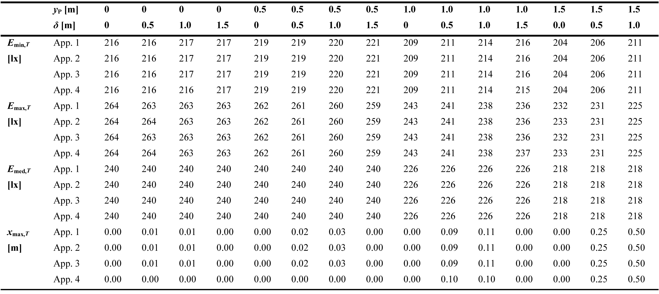
Table 2. Obtained values of E_min,T, E_max,T, E_med,T, and x_max,T using the four approaches in the configuration with BZ1 LID type.

Table 3

Table 3. Obtained values of E_min,T, E_max,T, E_med,T, and x_max,T using the four approaches in the configuration with the BZ5 LID type.

Table 4

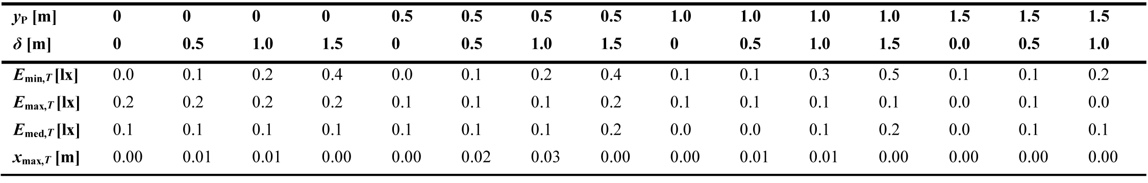
Absolute differences between the largest and smallest values of Emin,T, Emax,T, Emed,T, and xmax,T obtained with the four approaches in the configuration with BZ1 LID type.

Table 4. Absolute differences between the largest and smallest values of E_min,T, E_max,T, E_med,T, and x_max,T obtained with the four approaches in the configuration with BZ1 LID type.

Table 5

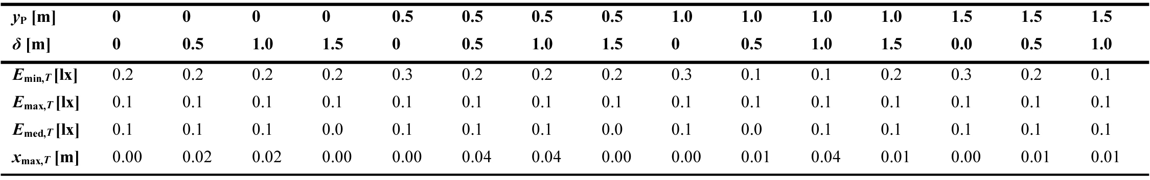
Table 5. Absolute differences between the largest and smallest values of E_min,T, E_max,T, E_med,T, and x_max,T obtained with the four approaches in the configuration with BZ5 LID type.

The greatest difference between illuminances obtained using the four approaches is 0.5 lx, achieved for E_min,T in the configuration with y_P = 1 m, δ = 1.5 m, BZ1 type. Meanwhile, the greatest difference between x_max,T values from all approaches is 0.04 m, i.e. less than half of the interval between calculation points, achieved in the configuration with (y_P, δ) = (0.5 m, 0.5 m); (0.5 m, 1.0 m); and (1 m, 1 m); all with BZ5 type. The greatest differences between E_max,T values and between E_med,T values from all approaches are found to be only 0.2 lx, hence practically no difference at all.

To give further illustrations, Fig. 9 displays the plots of E_T(x) with respect to x ∈ [–1.5 m, 4.5 m], obtained using the four approaches, in the configuration with y_P = 1 m, δ = 1 m, BZ1 type; and y_P = 1 m, δ = 1.5 m, BZ5 type. It is observed that the resulting graphs are perfectly sinusoidal and nearly identical with each other, suggesting a good agreement between all approaches, either with or without applying the phasor addition, regardless of the selected configuration.

Figure 9

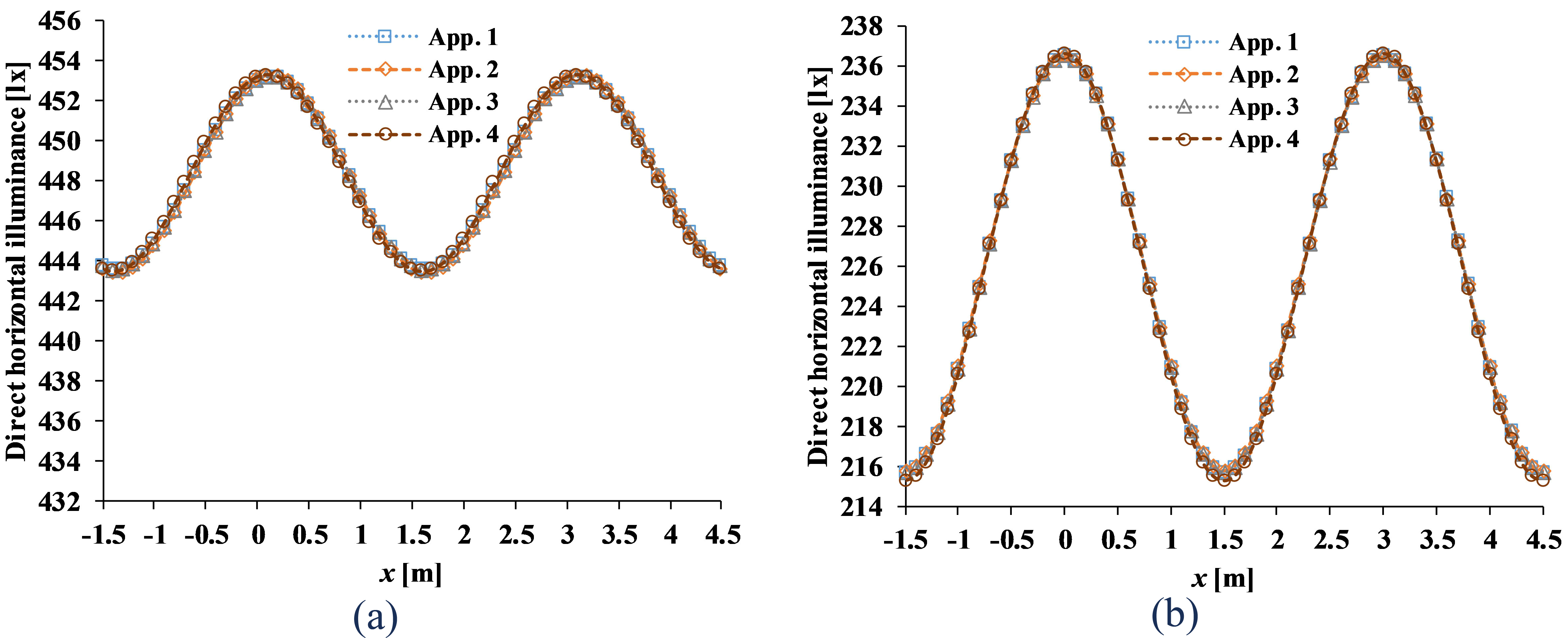
Fig. 9. Total direct horizontal illuminance E_T(x) obtained using Approach 1 until 4, in the configuration with (a) y_P = 1 m, δ = 1 m, BZ1 type; (b) y_P = 1 m, δ = 1.5 m, BZ5 type.

4.2. Sensitivity analysis

Table 6 displays the SRC (β ’) of each input variable in Equation (20), based on the sensitivity analysis results. The adjusted coefficient of determination (R²_adj) of the linear model of ΔE ’ is 0.921, and thus is sufficiently high to ensure reliable results.

Table 6

Table 6. SRC (β ’) of each input variable based on the sensitivity analysis results.

The largest SRC in the ΔE ’ sensitivity model is 0.899, obtained for n’. In other words, the choice of LID type of the source can significantly affect ΔE. When n = 1 (BZ5 type), ΔE is relatively small so that the fluctuation between E_max,T and E_min,T may be unnoticeable, because the sources’ LID is wide (120° beam angle) and thus create smaller contrast within points along the calculation row. Conversely, when n = 5 (BZ1 type, 66° beam angle), the fluctuation may be noticeable, since the narrow LID corresponds to smaller beam angle, yielding a greater contrast along the row. For any n values in between, the resulting performance can be estimated accordingly due to the linear behaviour of the variables.

Meanwhile, the lateral position of the calculation row (y_P) and spatial phase difference (δ) are relatively less influential on the fluctuation (SRC = –0.341 and –0.131 respectively). The impacts from both variables are negative, meaning that the larger the y_P and δ values, the smaller the spatial contrast. It should be noticed however that the variation of y_P and δ is periodic, so that the predicted effects only apply within the range between 0 and λ/2. Beyond that range, the effect would be symmetrical and not be continuously increasing (or decreasing).

Figure 10

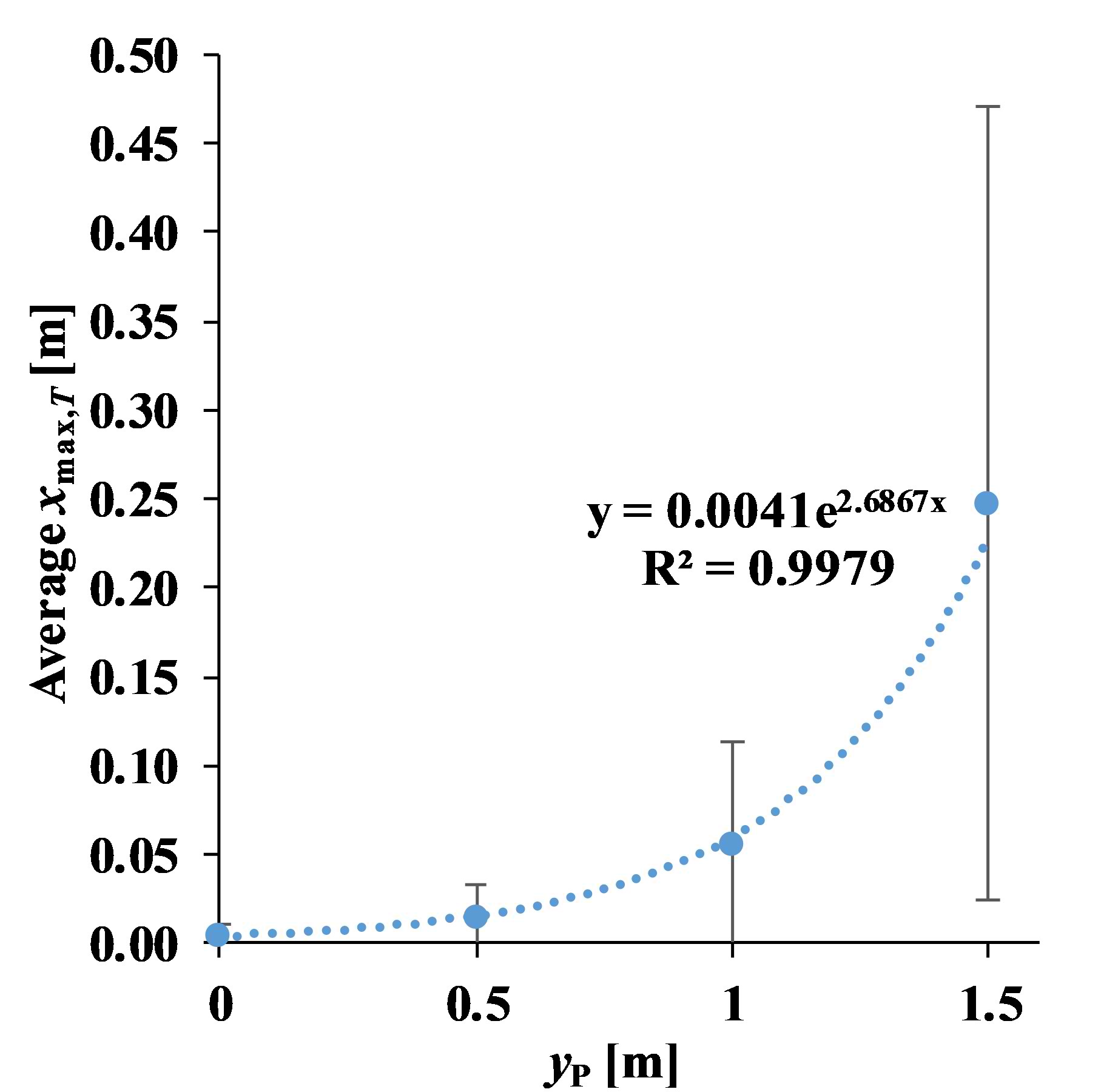
Fig. 10. Average x_max,T in all configurations against y_P; error bars denote the standard deviations.

While the ΔE ’ sensitivity model is highly linear, the x ’_max,T model is not (R²_adj = 0.321); so that the results cannot be held reliable. It is noticed however that the largest SRC in that model is of y_P’ (0.619). Thus, an additional analysis is performed by plotting the average x_max,T in all configurations against the y_P values. Figure 10 displays the resulting plot, suggesting a logarithmic relation (R² = 0.998) between both variables. The standard deviation from the average values, however, can be considerably large, particularly for y_P = 1.5 m. The large deviations can be attributed to the significant difference of both LID types, which can be observed from pattern comparison as follows.

The sinusoidal patterns of E_T(x) in all configurations are compared to each other in Fig. 11, with respect to x ∈ [–1.5 m, 4.5 m]. With the same I₀ value of 1800 cd for both LID types, the resulting E_T(x) values for BZ5 are approximately twice those for BZ1. The E_T(x) fluctuations (i.e. E_max – E_min = 2E_o) due to BZ1 can be as large as 50 lx, whereas those due to BZ5 are not found larger than 15 lx. This is again due to the beam angles associated with the LID pattern, where larger n values (as in BZ1) correspond to narrower light distribution, hence greater spatial contrast. In general, it explains why the LID types are deemed significant in influencing ΔE in the sensitivity analysis. Meanwhile, the impact of y_P and δ variations on ΔE patterns are not consistent across all configurations. In the BZ5 type, ΔE values tend to be similar regardless the y_P and δ. However, in the BZ1 type, larger ΔE values are found for y_P = 0 and 0.5 m; while for y_P = 1 and 1.5 m, the values tend to become smaller.

Figure 11

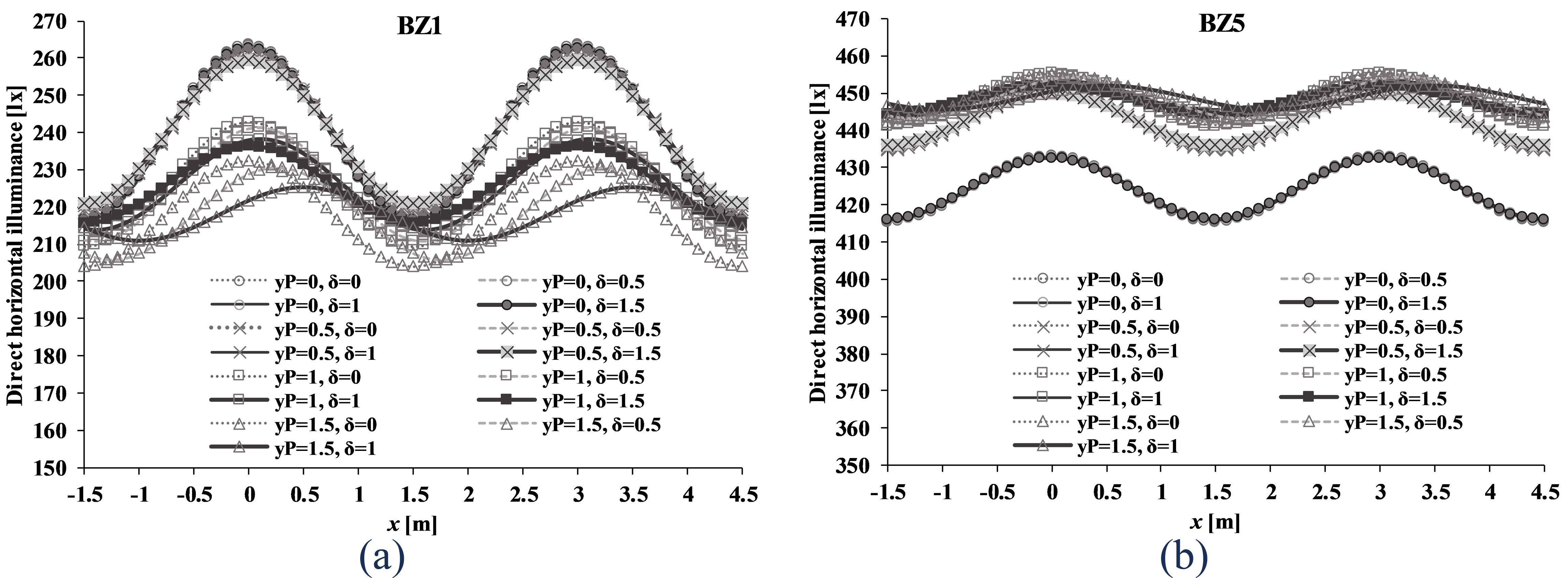
Fig. 11. Total direct horizontal illuminance E_T(x) in all configurations with (a) BZ1 and (b) BZ5 LID type.

With respect to x_max,T, it is observed that for 0 ≤ y_P ≤ 1 m, the x_max,T values are close to zero, meaning that the maximum E_T(x) are located near any individual source in the first array. The behaviour of x_max,T due to variation of y_P is however not linear, as described in Fig. 10. When y_P = 1.5 m, i.e. halfway the lateral distance between both arrays (Y), the shift of x_max,T due to varying δ is more noticeable, up to 0.5 m. In the scenarios with y_P = 1.5 m and δ = 1 m, not only the location of maximum E_T(x) shifts to the right, but also the ΔE tends to get smaller, suggesting less fluctuating pattern. When y_P = δ = 1.5 m, there will be no fluctuations at all (ΔE = 0), thus a completely uniform spatial pattern is achieved along the particular row.

As an alternative to visualise the results, several samples of the scenes with BZ1, δ = 0; BZ1, δ = 1.5 m; BZ5, δ = 0; and BZ5, δ = 1.5 m are modelled and simulated in DIALux 4.12 [28,29], with light loss factor of 1.0. In addition, to visualise the illuminance distribution on arbitrary vertical planes, two parallel black walls are introduced at y = –0.5 m and 3.5 m (i.e. 0.5 m beyond each sources’ array). The resulting false colour images showing direct illuminance distribution on the surfaces in those scenes are displayed in Fig. 12. Note that the same illuminance scale, between 150 and 550 lx, are employed in those four scenes.

Figure 12

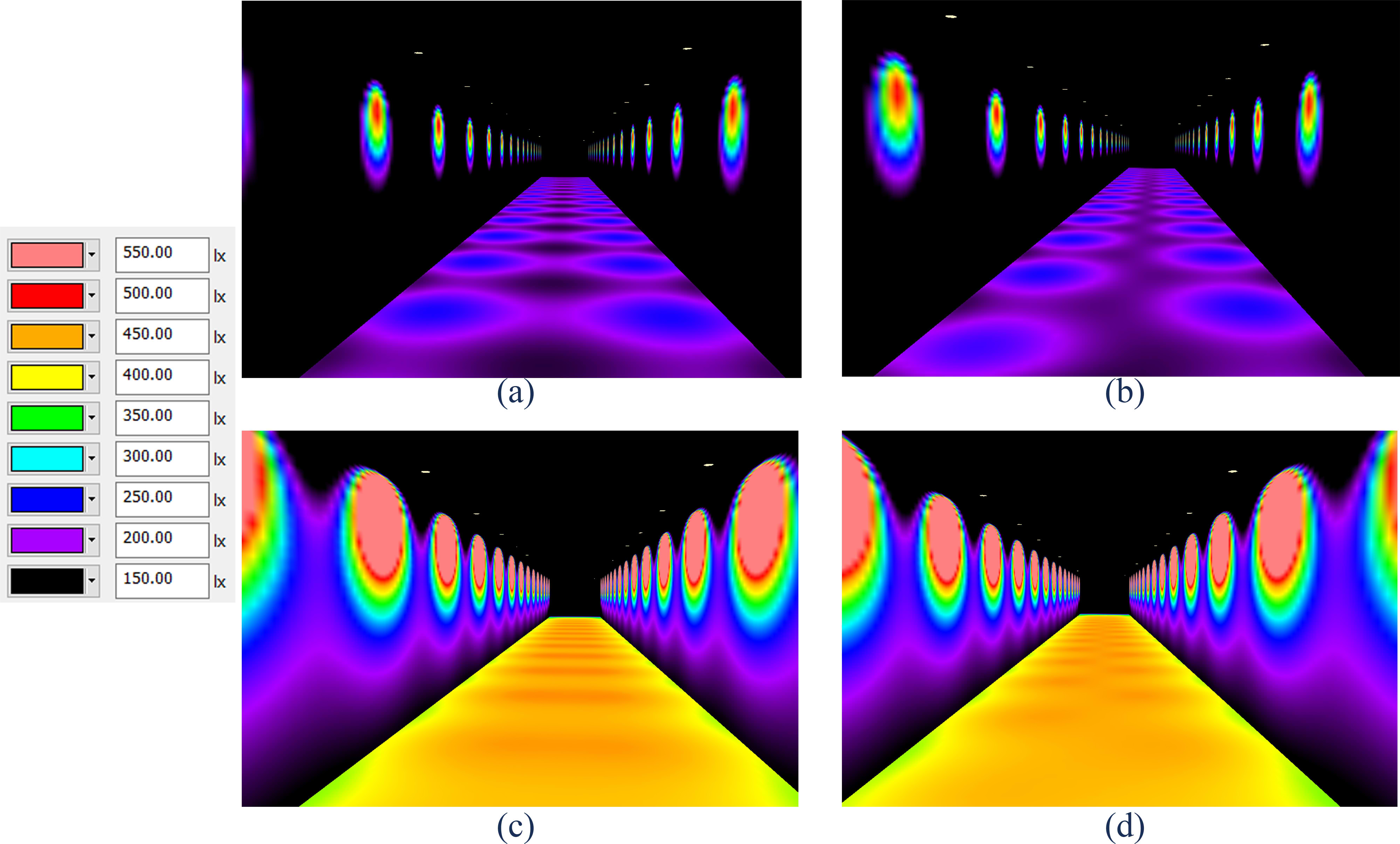
Fig. 12. False colour images of direct illuminance on surfaces in scenes with (a) BZ1, δ = 0, (b) BZ1, δ = 1.5 m, (c) BZ5, δ = 0, (d) BZ5, δ = 1.5 m, simulated in DIALux 4.12.

It is observed that while the maximum luminous intensity I₀ = 1800 cd is constant for both BZ types, the maximum E_P values in the BZ1 scenes are smaller than those in the BZ5 scenes, due to the wider LID in the latter. For the same reason, the E_P variations in the BZ5 scenes are also less visible than those in the BZ1 scenes. Regardless of the δ values, the highest spatial contrast in the BZ1 scenes are found between the points beneath the sources and those on the middle row. Nevertheless, increasing the δ value up to 1.5 m (= λ/2) may reduce this contrast, relative to δ = 0. In the BZ5 scenes, shifting the δ value is not expected to dramatically change the visual observation of the horizontal surface.

5. Discussion

The following remarks can be made regarding the phasor method proposed in Section 2 as Approaches 1 and 2. Both approaches can be employed in the situation where the individual E_P from the source is known or can be determined. Approach 2 is relatively simpler than Approach 1, which requires a certain sinusoidal regression calculator; but if there are too few discrete E_P data, the estimation of x_max value in Approach 2 may be incorrect, because the actual x_max value may be located between (i.e. not exactly on) the observed calculation points.

Meanwhile, the direct observation of E_T(x) data as in Approaches 3 and 4 can be performed only if such data are available, for instance in an actual installation. Approach 4 is simpler than Approach 2, with the same reason as in Approach 2 to Approach 1. Again, Approach 4 may however be less accurate if the actual x_max value lies between the observed calculation points. Of course, the individual E_P from the two sources’ arrays can be simply added to each other to obtain E_T(x); but the idea is to determine the optimum configuration of both arrays without having to perform the ‘trial and error’ approach. By showing that the results obtained using all four approaches are similar to each other, the concept of phasor method to predict the E_T(x) in this case is verified.

In turn, one may still question the usefulness of such concept in lighting design. To answer that, it is first to be understood that an engineering design process requires a known relation between input (design parameters) and output variables (performance indicators). Once the values of the output variables have been defined, for instance based on standards, regulations, or user requirements, the designer shall be able to determine the required input variables values. In this case, the resulting E_T(x) pattern is the desired output, whereas the geometrical variables are to be designed accordingly.

An obvious example would be the case to determine the position of calculation row having uniform pattern of E_T(x), which can be achieved by setting y_P = Y/2 and δ = λ/2. Since Y and λ cannot be zero because both arrays and adjacent sources must be separated by a finite distance, δ cannot be zero either. When the arrays configuration is staggered with δ = λ/2, i.e. half the interval between adjacent sources in each array, the E₁(x) and E₂(x) patterns cancel each other out with respect to E_med, as mentioned in Section 3. Applying a perfectly aligned configuration (δ = 0), instead of the staggered one, shall not yield a uniform pattern in the middle row. Of course, these observations are valid with the underlying assumptions, e.g. the sources in each array are identical and have a cosine-like LID type, the interval λ is constant for both arrays, and only direct illuminances are considered. Nevertheless, the general idea should be visible here.

While the case of y_P = Y/2 is quite intuitive due to symmetry, the case of arbitrary y_P values (0 < y_P < Y/2) may be less obvious, so that the configuration of both arrays should be designed properly. In that case, one can start with the desired sinusoidal pattern of E_T(x), by defining the intended E_min,T, E_max,T, E_med,T, and x_max,T values, so that E_o_,T, k (= 2π/λ), and ϕ_T coefficients can be determined. Next, the contribution from a single array to the calculation row may be determined, so that E_o_,1 can be defined, whereas k is already a constant and ϕ₁ can be set to zero with respect to the first array. Equations (9) and (10) can therefore be applied simultaneously to determine E_o_,2 and ϕ₂. Once E_o_,2 and ϕ₂ are known, the location of the second array can be determined.

Equivalently, one can construct the phasor diagram as in Fig. 6 and proceed with conducting the analysis to obtain E_o_,2 and ϕ₂ (Fig. 13). From the diagram, one can write: tan ϕ₂ = E_o_,T sin ϕ_T / (E_o_,T cos ϕ_T – E_o_,1) and then solve for ϕ₂. Furthermore, since E_o_,2 sin ϕ₂ = E_o_,T sin ϕ_T, one can also solve for E_o_,2. Again, the advantage of using phasor method with complex notation is demonstrated here, which is expected to help in understanding the superposition phenomenon and in achieving the intended E_T(x) pattern.

Figure 13

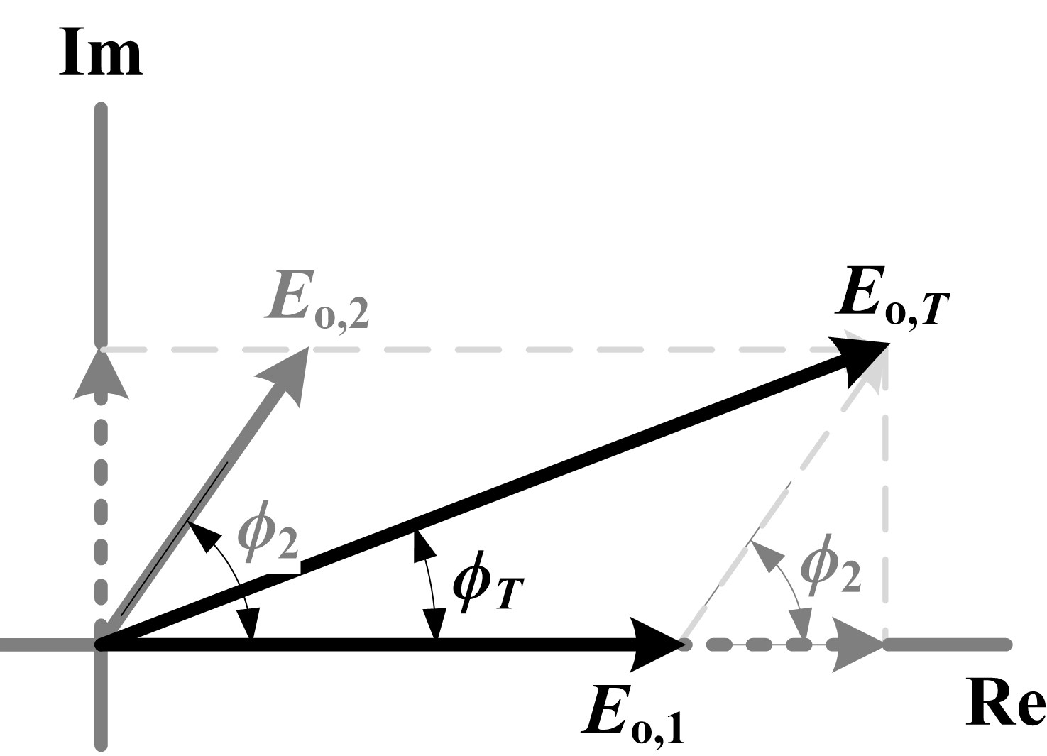
Phasor diagram to determine Eo,2 and ϕ2 from the defined Eo,T, ϕT, Eo,1, and ϕ1 (= 0).

Fig. 13. Phasor diagram to determine E_o_,2 and ϕ₂ from the defined E_o_,T, ϕ_T, E_o_,1, and ϕ₁ (= 0).

As mentioned earlier, several main assumptions are required in the entire concept. First, all sources should possess a cosine-like LID, so that the resulting E₁(x), E₂(x), and E_T(x) all reveal sinusoidal patterns. Such LID type is reasonable for typical downlight, point-source luminaires for indoor applications. Thus, the proposed cases may be applicable for interior spaces with parallel and periodic arrays of downlights and with little reflections from the surrounding surfaces, e.g. large reading halls in libraries (as in Fig. 1), auditoriums, theatres, or galleries. It is also possible to find applications in outdoor scenes, as in pedestrian or small residential lighting. Meanwhile, large street lighting luminaires typically have a batwing type of LID, which will yield a sawtooth-like, instead of sinusoidal, pattern of illuminance.

The second main assumption is that both arrays have a constant spatial wavelength λ, which is necessary to enable the use of phasor diagram, where one can put the term e^jkx in Equation (8) aside and recall it later once the superposition has been done. In cases where λ from both arrays are different, the cosine terms shall be added individually. In turn, it should be possible to decompose the combined pattern of E_T(x) using Fourier series expansion, to reveal the individual wavelengths (or frequencies). This is beyond the scope of this article but can be definitely considered for future studies.

Finally, to give another perspective on the applicability of the proposed concept, it is worthwhile to thoroughly read the proposal of Cuttle et al. [12,23,24] regarding the appearance-based, perceived adequacy of illumination (PAI), and the eventual reception of his proposal during the past decade. While they argue that horizontal illuminance is not necessarily related with PAI and spatial brightness [12], some (perhaps many) will keep saying that horizontal workplane illuminance is still very much what matters in the design practice [30]. In this current study, though still based on horizontal illuminance, the resulting patterns are never expected to be uniform (except for the special case of y_P = Y/2 and δ = λ/2), and thus can be related to some extent with the concept of target/ambience illuminance ratio (TAIR) [24,30]. For instance, though not exactly the same, the E_min can be compared in analogy with the ambient illuminance, whereas E_max with the target illuminance.

As a follow-up of this current study, further investigations are suggested on more scenarios involving sinusoidal patterns of illuminance in various realistic situations, for instance in large halls or residential roads. Furthermore, since this study only considers regularly-spaced arrays of sources, scenarios in future studies can also be extended to irregularly-spaced arrays. The proposed phasor method in this study is thus expected to become a tool to better understand the physical phenomena of light superposition from parallel arrays of sources, and eventually to refresh the design practice in such cases.

6. Conclusion

Direct horizontal illuminance along a calculation row (E_T(x)) due to two parallel and periodic arrays of large numbers of identical light sources, with a cosine-like luminous intensity distribution (LID) type, reveals a sinusoidal pattern that contains several important information. Four different approaches, including the use of phasor method, are employed to verify the concept of adding the sinusoidal pattern of direct illuminance from both arrays. Examples of configuration with BZ1 or BZ5 LID type are introduced, as described in Section 3. A very good agreement, with differences of ≤ 0.5 lx for the illuminances (E_max,T, E_min,T, E_med,T) and ≤ 0.04 m for the position of maximum illuminance (x_max,T), is found between all approaches in all configurations. The proposed concept is thus verified.

Based on the sensitivity analysis, the choice of LID type significantly affects ΔE, which is the ratio between (E_max,T – E_min,T) and E_med,T. For BZ5 type, ΔE is relatively small so that the illuminance fluctuation may be unnoticeable, because the sources’ LID is wide (120° beam angle) and thus create smaller contrast within points along the calculation row. For BZ1 type, the fluctuation may however be noticeable, since the narrow LID corresponds to smaller beam angle, yielding greater spatial contrast.

Meanwhile, the impact of lateral position of the calculation row (y_P) and the spatial phase difference (δ) on ΔE patterns are inconsistent. In the tested scenarios, for 0 ≤ y_P ≤ 1 m, the maximum E_T(x) are located near any individual source in the first array. The behaviour of x_max,T due to variation of y_P is however not linear. When y_P = 1.5 m, i.e. halfway the lateral distance between both arrays (Y), the shift of x_max,T due to varying δ is more noticeable. In the scenarios with y_P = 1.5 m and δ = 1 m, not only the location of maximum E_T(x) shifts to the right, but also the E_T(x) fluctuation becomes less. When y_P = δ = 1.5 m, a completely uniform spatial pattern with no fluctuations is achieved along the particular row. Overall, the advantage of using phasor method with complex notation has been demonstrated, which is expected to help in understanding the superposition phenomenon of sinusoidal pattern of illuminance, and in achieving the desired spatial contrast.

Acknowledgement

This research is supported by the Institute of Research and Community Service of Institut Teknologi Bandung (LPPM ITB), under the P3MI 2020 research scheme.

Contributions

R. A. M. designed the research framework, performed the computation and simulation, and wrote the manuscript. At. reviewed and co-wrote the manuscript.

Declaration of competing interest

The author declares that there is no conflict of interest.

References

J.H. Lambert, Photometria, sive de Mensura et Gradibus Luminis, Colorum et Umbrae, Eberhard Klett, Augsburg, 1760.
D.L. DiLaura, K.W. Houser, R.G. Mistrick, G.R. Steffy (eds.), The Lighting Handbook: Reference and Application, 10th Edition, Illuminating Engineering Society, New York, 2011.
P.R Boyce, Editorial: Illuminating engineering rises from the grave, Lighting Research and Technology 51 (2019) 487–487. https://doi.org/10.1177/1477153519852246
C.E. Ochoa, M.B.C. Aries, J.L.M. Hensen, State of the art in lighting simulation for building science: a literature review, Journal of Building Performance Simulation 5 (2012) 209–233. https://doi.org/10.1080/19401493.2011.558211
Z. Huang, A. Sanderson, Light field modelling and interpolation using Kriging techniques, Lighting Research and Technology 46 (2013) 219–237. https://doi.org/10.1177/1477153512473996
A.A. Baloch, P.H. Shaikh, F. Shaikh, Z.H. Leghari, N.H. Mirjat, M.A. Uqai, Simulation tools application for artificial lighting in buildings, Renewable and Sustainable Energy Reviews 82 (2018) 3007–3026. https://doi.org/10.1016/j.rser.2017.10.035
R.H. Simons, A.R. Bean, Lighting Engineering: Applied Calculations, Architectural Press, Oxford, 2001.
C.F. Reinhart, T. Dogan, D. Ibarra, H.W. Samuelson, Learning by playing – teaching energy simulation as a game. Journal of Building Performance Simulation 5 (2012) 359–368. https://doi.org/10.1080/19401493.2011.619668
I. Beausoleil-Morrison, Learning the fundamentals of building performance simulation through an experiential teaching approach, Journal of Building Performance Simulation 12 (2019) 308–325. https://doi.org/10.1080/19401493.2018.1479773
J.A. Lynes, Designing for contrast rendition, Lighting Research and Technology 14 (1982) 1–18. https://doi.org/10.1177/096032718201400101
S. Rockcastle, M. Amundadottir, M. Andersen, Contrast measures for predicting perceptual effects of daylight in architectural renderings, Lighting Research and Technology 49 (2016) 882–903. https://doi.org/10.1177/1477153516644292
J. Duff, K. Kelly, C. Cuttle, Perceived adequacy of illumination, spatial brightness, horizontal illuminance and mean room surface exitance in a small office, Lighting Research and Technology 49 (2017) 133–146. https://doi.org/10.1177/1477153515599189
J.M. Monteoliva, A. Villalba, A. Pattini, Daylighting metrics: an approach to dynamic cubic illuminance, Journal of Daylighting 5 (2018) 34–42. https://doi.org/10.15627/jd.2018.6
V.W.L. Lo, K.A. Steemers, Methods for assessing the effects of spatial luminance patterns on perceived qualities of concert lighting, Lighting Research and Technology 52 (2019) 106–130. https://doi.org/10.1177/1477153519841098
F. Selim, S.M. Elkholy, A.F. Bendary, A new trend for indoor lighting design based on a hybrid methodology, Journal of Daylighting 7 (2020) 137–153.
A. Lauria, S. Secchi, L. Vessella, Visual wayfinding for partially sighted pedestrians – The use of luminance contrast in outdoor pavings, Lighting Research and Technology 51 (2018) 937–955. https://doi.org/10.1177/1477153518792978
Y. Jiang, S. Li, B. Guan, G. Zhao, D. Boruff, L. Garg, P. Patel, Field evaluation of selected light sources for roadway lighting, Journal of Traffic and Transportation Engineering (English Edition) 5 (2018) 372–385. https://doi.org/10.1016/j.jtte.2018.05.002
D.M. Kretzer, High-mast lighting as an adequate way of lighting pedestrian paths in informal settlements?, Development Engineering 5 (2020) 100053. https://doi.org/10.1016/j.deveng.2020.100053
S. Fotios, C. Robbins, Research Note: Describing average illuminance for P-class roads, Lighting Research and Technology, in press. https://doi.org/10.1177/1477153520911193
D. Cetegen, J. Veitch, G. Newsham, View size and office illuminance effects on employee satisfaction, Proceedings of Balkan light, Ljubljana, Slovenia (2008).
D. Tiller, J. Veitch, Perceived room brightness: pilot study on the effect of luminance distribution, Lighting Research and Technology 27 (1995) 93–101. https://doi.org/10.1177/14771535950270020401
K. Wymelenberg, M. Inanici, A study of luminance distribution patterns and occupant preference in daylit offices, Proceedings of PLEA 2009 - the 26th conference on passive and low energy architecture, Quebec City (2009).
C. Cuttle, Towards the third stage of lighting profession, Lighting Research and Technology 42 (2010) 73–93. https://doi.org/10.1177/1477153509104013
C. Cuttle, A new direction for general lighting practice, Lighting Research and Technology 45 (2013) 22–39. https://doi.org/10.1177/1477153512469201
W.R. Stevens, Building Physics: Lighting – Seeing in the Artificial Environment, Pergamon Press, Exeter, 1969.
J.A. Lynes, Does the British Zonal System have a future?, Lighting Research and Technology 11 (1979) 150–153. https://doi.org/10.1177/14771535790110030201
Stats.Blue, Sinusoidal Regression Calculator, Available online at: http://stats.blue/Stats_Suite/sinusoidal_regression_calculator.html. 2018. zzzzzz
DIAL GmbH. DIALux. Available online at: https://www.dial.de/en/dialux/.
R.A. Mangkuto, Validation of DIALux 4.12 and DIALux evo 4.1 against the analytical test cases of CIE 171:2006, LEUKOS 12 (2016) 139–150. https://doi.org/10.1080/15502724.2015.1061438
C. Cuttle, Lighting by Design. 2nd Edition, Routledge, London, 2008.

Get PDF (5.6 MB)

SHARE ON