

Omar Kanaan Al Basri1,*, Fayrooz Kanaan Nori2, Mohammed Abdulridha Hussein3
Author affiliations
- 1Collage of engineering, Al Karakh University of Sciences KUS, Baghdad, Iraq
- 2College of Applied Sciences, Fallujah University, 31002, Fallujah, Anbar, Iraq
- 3Department of environmental science, Al Karakh University of Sciences KUS, Baghdad, Iraq
*Corresponding author.
- omar.k84@kus.edu.iq (O. K. A. Basri)
- fayrouz.kanaan@uofallujah.edu.iq (F. K. Nori)
- Mohammed_it@mtu.edu.iq (M. A. Hussein)
History: Published online 19 November 2026
Copyright: © 2026 The Author(s). Licensee Solarlits Limited (Hong Kong). This is an open access article distributed under the terms and conditions of the Creative Commons Attribution 4.0 License.
Citation: Omar Kanaan Al Basri, Fayrooz Kanaan Nori, Mohammed Abdulridha Hussein, Voltage Stability Analysis of Low-Voltage Distribution Networks with High Penetration of Rooftop PV Systems, Journal of Daylighting, 13:2 (2026) 770-792. doi: 10.15627/jd.2026.41
Abstract
The paper presents a study on the effect of increasing rooftop PV penetration on voltage stability of low-voltage (LV) radial distribution feeders. A 12-bus European-style LV feeder modeled using the CIGRE benchmark parameters with NAYY 4×35 mm² aluminium underground cable is considered at 400 V/50 Hz. The Backward-Forward Sweep (BFS) algorithm is applied for load flow analysis under six different PV penetration cases from 0% to 100% (the PV penetration factor ρ is defined throughout as the fraction of the feeder’s aggregate rooftop-PV capacity that is in service, each of the eleven load buses being equipped with a PV unit rated at 110% of its own peak active load, so that ρ = 100% corresponds to 62.70 kWp of installed PV against a 57.00 kW feeder peak demand) with 24-hour residential load and clear-sky solar irradiance data. The voltage stability indices like Fast Voltage Stability Index (FVSI), Voltage Stability Index (VSI) and Voltage Deviation Index (VDI) are used and the results are compared against the EN 50160 limit for power quality. It is observed that the PV penetration decreases the active power losses gradually and up to 41.4% as compared to the base case. However, it also causes an overvoltage violation at Bus 11, where the maximum bus voltage reaches 1.1092 pu, exceeding the EN 50160 upper limit of 1.10 pu by 0.92%. VDI shows a non-monotonic behavior with the PV penetration and has its minimum value of 0.0631 pu at 60% penetration level, thus representing the same as an optimal operating point. Furthermore, FVSI and VSI indicate that voltage collapse is not the issue of concern in all the cases, while the power quality is the new limit. The power-flow implementation is verified against three relations that follow analytically from the model equations, and a mitigation assessment shows that, because the resistance-to-reactance ratio of the NAYY 4×35 mm² cable is 10.59, reactive Volt-VAr control is an intrinsically inefficient countermeasure on this feeder — restoring compliance by reactive absorption alone would require an inverter apparent-power rating 1.93 times the active rating — whereas a 0.025 pu reduction of the transformer set-point in the midday hours, a 15.5% curtailment of the exported surplus, or distributed battery storage each restore full EN 50160 compliance at 100% penetration.
Keywords
Rooftop photovoltaic, Low-voltage distribution network, Voltage stability, FVSI
Nomenclature
| BESS | Annual Sunlight Exposure |
| BFS | Climate-Based Daylight Modeling |
| CIGRE | European Standard |
| DER | Indoor Environmental Quality |
| DG | Global Alliance for Buildings and Construction |
| DS | Honeybee |
| FVSI | International Glazing Database |
| IEEE | International Energy Agency |
| LV | Illuminating Engineering Society |
| ML | Ladybug |
| MV | Lawrence Berkeley National Laboratory |
| OLTC | Lighting Energy (Annual Consumption) |
| PF | Leadership in Energy and Environmental Design |
| PQ | Lighting Power Density |
| PV | Multi-Criteria Decision Making |
| UPQC | Quality of View |
| VDI | Renewable Energy Policy Network for the 21st Century |
| VSI | Spatial Daylight Autonomy |
| ZIP | Technique for Order Preference by Similarity to Ideal Solution |
1. Introduction
Global rooftop photovoltaic (PV) markets have boomed in the last decade in European, Australian and Asian regions due to low costs of solar panels, the feed-in tariff schemes and consumer’s awareness towards green energy [1]. Consequently, the conventional mode of power distribution system (DS) from centralized production to the end-users has been disrupted and an increasing amount of distributed generation (DG) is observed [2], where residential customers with rooftop PV systems contribute to the power distribution. While supporting the decarbonisation efforts [3], this trend of decarbonisation also presents new technical challenges for the network operator to maintain a power quality (PQ) that complies with the regulations [4]. In this paper, we aim to analyse the impact of PV rooftop systems on voltage profile at residential low-voltage (LV) distribution system in terms of the EN 50160 standard [5].
Voltage variations are to be expected due to reverse power flows during solar peak times especially in the radial grid with high resistive R/X ratio. The EN 50160 standard of voltage stability limits the supply voltage to be within ±10% of the rated voltage [6]. High PV penetration along with lack of any reactive power compensation, the voltage at a distant node from the substation may violate this undervoltage regulation [7]. In the mornings and evenings when the residential load peaks, the reverse power flow ceases, but the inability to meet the local power demand causes the undervoltage [8]. Therefore, both overvoltage and undervoltage due to PV rooftop systems may be a significant concern to the power utility in terms of network planning and investment in the grid reinforcement or voltage regulation devices [9].
The impact of PV on the PV penetration has been widely studied in the literature. However, most of the work is either focused on medium-voltage (MV) or single radial feeders which do not resemble the actual branched topology of LV systems in Europe [10]. Moreover, very few works have quantified the impact of PV penetration on the LV feeder voltage profile by computing FVSI, VSI and VDI indices in the same simulation by considering a full 24 h operation window [5]. With the help of a 12-bus CIGRE LV radial feeder, this work comprehensively studies the voltage stability issue of PV rooftop systems over a penetration range of 0%, 20%, 40%, 60%, 80% and 100% by considering FVSI, VSI, VDI indices. In doing so, it also enables to understand the effect of FVSI, VSI, VDI on LV feeder over the whole day and at what penetration limit the PV systems in the LV feeder cause EN 50160 violations.
The distinct diagnostic value of tracking FVSI, VSI and VDI concurrently, rather than relying on voltage-deviation screening or on a single conventional stability metric, warrants explicit statement, since the three indices answer different questions about the same operating point and can in principle disagree. FVSI is a branch-level, reactive-power-driven measure of proximity to the maximum-loadability point of a line, and it is sensitive to the reactive stress carried by individual branches. VSI is a receiving-end measure that retains both the active and the reactive flow terms and therefore responds to the total branch loading rather than to its reactive part alone. VDI, by contrast, is not a stability measure at all: it is a purely nodal power-quality measure of the worst per-unit excursion from nominal, and it is blind to how much loadability margin remains. Evaluating the three together allows the operating limit of the feeder to be attributed unambiguously to its physical cause rather than merely detected.
That attribution is the substantive result of this study. Screening on voltage deviation alone would have identified the EN 50160 breach at full penetration but could not have excluded a simultaneous erosion of the collapse margin, and would therefore have left open the possibility that network reinforcement rather than voltage control was required. Screening on the collapse indices alone would have declared the feeder unconstrained across the whole penetration range and would have missed the hosting-capacity limit entirely. Only the concurrent evaluation establishes the quantitative separation reported here — FVSI never exceeding 0.0798 and VSI never falling below 0.706 pu, that is, margins in excess of 92% and 70% respectively, while the statutory voltage band is breached — and it is that separation, resolved hour by hour and across a controlled penetration sweep, which converts a qualitative expectation into a design rule: on a resistive LV feeder the collapse indices inherited from transmission practice are diagnostically inert, and hosting capacity is set by the statutory voltage band.
The specific contributions of the paper are therefore: (i) a 24-hour, six-scenario penetration sweep on a CIGRE-parameterised 12-bus European LV feeder in which FVSI, VSI and VDI are evaluated simultaneously at all 144 operating points; (ii) identification of a voltage-quality-optimal penetration of 60%, at which VDI is minimised, that is distinct from the loss-optimal penetration of 80%; (iii) determination of the EN 50160 hosting-capacity limit of the feeder, resolved by bus, by hour and by violation duration rather than reported as a single count; (iv) a closed-form assessment of Volt-VAr control, transformer tap adjustment, active-power curtailment, reconductoring and battery storage as mitigation measures for a high-R/X LV feeder; and (v) an explicit sensitivity and limitation analysis covering irradiance variability, load stochasticity, load modelling, feeder geometry and phase unbalance.
3. Proposed methodology
The paper proposes a simulation-based methodology for voltage stability assessment of a 12-bus European LV type radial distribution network with six cases of rooftop PV penetration levels. The proposed methodology consists of modeling the network, 24-hour power flow calculations and multi-index stability analysis by comparing it to EN 50160 power quality requirements.
3.1. Network model and system parameters
The test network is a 12-bus radial feeder based on the CIGRE low-voltage benchmark, with 400 V (line-to-line) and 50 Hz. It consists of the main feeder with seven buses (B0–B6) in series of 100 m segments and two laterals (Lateral-1: B2–B7–B8 of 150 m segments, and Lateral-2: B4–B9–B10–B11 of 150 m segments). Bus B0 is the slack bus that corresponds to the MV/LV distribution transformer, whose secondary voltage set-point is held at 1.05 pu (typical on-load tap changer (OLTC) offset applied by utilities to cover the nominal load drop) that otherwise would have been at 1 pu in all other cases. Note that this actually makes the nominal overvoltage more severe under high PV generation.
The whole network has its branches modelled by NAYY 4×35 mm2 aluminium underground cable with the following per-unit-length parameters [24]: r = 0.868 Ω/km, x = 0.082 Ω/km.
The base quantities used for per-unit normalisation are: Sbase = 100 kVA, Vbase = 0.4 kV.
Branch impedance for a segment of length 𝐿 (in km) is computed as [25]:
Each load bus (B1–B11) has an associated residential load with a power factor of about 0.95 lagging. Active power injections vary between 4.0 and 6.0 kW/bus at peak. Thus, the total network peak demand is around 57 kW. In addition to the loads, each bus has a rooftop PV unit rated at 110% of peak load. This sizing is roughly in line with modern European and Australian residential solar sizing (inclusive of battery storage) [26]:
3.2. Daily load and solar irradiance profiles
The hourly load demand and clear-sky solar irradiance profiles are normalised to a 24 h horizon for the simulation. There is no external measured dataset. The input hourly time series for 𝐿(ℎ) and 𝐺𝑐𝑠(ℎ) are analytically synthesised to model the conditions expected for a representative European residential setting, in line with common CIGRE and IEEE normal load modelling conventions.
The load profile 𝐿(ℎ) exhibits a typical European double-peak residential shape: a morning peak at hour 7 (𝐿 = 0.70) associated with domestic morning routines and an evening peak at hour 19 (𝐿 = 1.00) linked to after-work household activity. Overnight, the load settles to a low-value plateau in the range 0.38–0.45 pu. The actual injected active and reactive power at bus 𝑏 at hour ℎ is [27]:
The bus load and pv rated power data are listed in Table 1. The clear-sky solar irradiance profile 𝑆(ℎ) is modelled as a Gaussian bell curve centred at solar noon (hour 13), active only between hours 6 and 20 [28]:
| Bus | Peak Active Load P_peak (kW) | Peak Reactive Load Q_peak (kVAR) | PV Rated Power P_PV,rated (kW) | Connected Lateral |
|---|---|---|---|---|
| B0 | — | — | — | Slack (Transformer) |
| B1 | 4.00 | 1.31 | 4.40 | Main feeder |
| B2 | 6.00 | 1.97 | 6.60 | Main feeder |
| B3 | 4.00 | 1.31 | 4.40 | Main feeder |
| B4 | 6.00 | 1.97 | 6.60 | Main feeder |
| B5 | 4.00 | 1.31 | 4.40 | Main feeder |
| B6 | 6.00 | 1.97 | 6.60 | Main feeder |
| B7 | 5.00 | 1.64 | 5.50 | Lateral-1 |
| B8 | 6.00 | 1.97 | 6.60 | Lateral-1 |
| B9 | 5.00 | 1.64 | 5.50 | Lateral-2 |
| B10 | 6.00 | 1.97 | 6.60 | Lateral-2 |
| B11 | 5.00 | 1.64 | 5.50 | Lateral-2 |
| Total | 57.00 | 18.70 | 62.70 | — |
The net active power injection at each bus accounts for the simultaneous load demand and PV generation, where 𝜌 ∈ {0, 0.20, 0.40, 0.60, 0.80, 1.00}denotes the PV penetration factor [18]:
Negative values of 𝑃_net represent a power flow from the bus back toward the transformer, which is the key effect causing a voltage rise at remote feeder buses during midday. 𝑄_net is assumed to be 𝑄_load since the PV inverters are modeled at unity power factor, which is the conservative legacy inverter assumption with no volt-VAR support capability.
Load representation. All bus loads in (4), (5) and (7) are modelled as constant-power (PQ) injections: the complex power Sⱼ = P_net(j) + jQ_net(j) that enters the backward sweep in (8) is held at its scheduled value irrespective of the solved bus voltage, so that no ZIP voltage-dependence is applied and no constant-impedance or constant-current component is included. This is the conservative choice for the present study, and it is conservative in both directions. A constant-power load draws increased current as the voltage falls, and therefore maximises the computed undervoltage at the evening demand peak; at the midday reverse-flow condition it holds the local load contribution constant as the voltage rises, and therefore does not attenuate the PV-driven voltage rise in the way that a constant-impedance component would.
Real aggregated residential demand is better represented by a ZIP model containing a substantial constant-impedance share, particularly for resistive heating, lighting and appliance loads. Substituting such a model would reduce both the computed evening undervoltage and the computed midday overvoltage, so the constant-power assumption bounds the voltage excursion from above at both ends of the daily cycle and cannot produce a violation that a ZIP model would not also produce in attenuated form. Because the EN 50160 exceedance found at 100% penetration is only 0.92%, the sensitivity of that margin to the load model is material rather than negligible, and it is quantified together with the other parameter sensitivities in Section 4.
3.3. Irradiance and load variability
The clear-sky profile defined by (6a)–(6b) is a deterministic upper envelope of the available solar resource. Used alone it is an idealisation in two distinct senses, and these must be separated because they act on different aspects of the result.
The first concerns the magnitude of the overvoltage. The clear-sky envelope maximises midday generation and therefore maximises reverse power flow and the resulting voltage rise. Any cloudy realisation of the same day reduces the instantaneous irradiance below the envelope and therefore produces a maximum bus voltage no greater than the clear-sky value. The overvoltage threshold identified in this study is consequently a worst-case rather than a typical-case result: it is the condition against which a compliance assessment must be designed, and in this respect the clear-sky assumption does not overstate the outcome by predicting violations that a variable day could not produce. What the assumption does overstate is the frequency and the duration of the violation. The eight bus-hour violations reported at 100% penetration are the count for a fully clear day; on a partly cloudy day the count is lower, and an annual expectation of violation-hours can only be obtained from a measured or synthetic irradiance year rather than from a single profile. This distinction between violation magnitude, which is bounded by the present analysis, and violation frequency, which is not, is quantified in the sensitivity analysis of Section 4.
The second concerns variability itself. A clear-sky profile has no high-frequency content and therefore cannot represent the ramp-driven phenomena — rapid voltage change, flicker, and the tap-changer and inverter control interactions they provoke — that transient cloud passage causes in high-PV LV feeders. These phenomena lie outside the scope of an hourly steady-state analysis by construction, since an hourly time step cannot resolve a cloud edge, which acts on a scale of seconds. The present study is a steady-state voltage-magnitude and stability-index study and makes no claim regarding dynamic power quality; assessing flicker and rapid voltage change would require sub-minute irradiance measurements together with a dynamic inverter model, and is listed as future work.
The load profile is subject to a symmetrical caveat. L(h) is an analytically synthesised deterministic double-peak shape representative of an aggregated European residential feeder and contains no stochasticity. Real aggregated demand at the scale of eleven buses and approximately 57 kW retains substantial diversity-driven random variation about its mean shape, and the coincidence factor of individual dwellings is materially below unity. High-resolution bottom-up stochastic demand models [29] show that the aggregate of a small number of dwellings has a coefficient of variation that does not vanish, and that the evening peak of an individual realisation can exceed the smooth mean profile appreciably. The practical implication for the present results is that the evening undervoltage reported at 0% penetration is a mean-profile value and that individual realisations would produce deeper minima, whereas the midday overvoltage, which occurs at the load trough where both absolute demand and absolute variability are smallest, is comparatively insensitive to load stochasticity. Since the binding constraint identified in this paper is the midday overvoltage, the deterministic load assumption affects the non-binding side of the result more than the binding side.
3.4. Backward-forward sweep power flow
The Backward-Forward Sweep (BFS) method is chosen for power flow calculations because it is better adapted to radial distribution networks with high R/X ratios. Newton-Raphson approaches result in ill-conditioned Jacobian matrices in this type of system. The BFS method is derived directly from the radial tree topology, does not require a matrix inversion, and reliably converges under both heavy load and reverse power flow situations. First, the network tree is parsed in breadth-first traversal order. Then, two sweeps are performed in sequence at each iteration. Backward Sweep — branch currents are calculated from leaf buses to the slack bus. For each bus 𝑗 with parent bus 𝑖, the branch current 𝐼_𝑖𝑗 is [12]:
where 𝑆𝑗 = 𝑃net(𝑗) + 𝑗𝑄net(𝑗) is the total apparent power at bus j.
Forward Sweep — bus voltages are updated from the slack bus toward the leaf buses. For each bus 𝑗 with parent bus 𝑖:
The slack bus voltage is fixed at:
Iterations continue until the maximum voltage magnitude change between successive iterations falls below the convergence tolerance:
Active and reactive power losses across branch 𝑖𝑗 are then computed as:
Total network active power loss at each hour is the sum over all 11 branches. The simulation executes 24 × 6 = 144 independent power flow solutions, one per hour per penetration level.
3.5. Balanced single-phase-equivalent representation and the effect of phase unbalance
The network is solved as a balanced single-phase equivalent: each bus load and each rooftop PV unit is represented by its three-phase aggregate, and the four-wire NAYY 4×35 mm² cable is reduced to a single positive-sequence series impedance. This is the standard representation for feeder-level hosting-capacity screening, and it is the representation in which the CIGRE benchmark parameters are published, but it is an idealisation and its consequences must be stated. European residential LV networks are inherently unbalanced, because rooftop inverters below approximately 4.6 kVA are conventionally connected single-phase and the phase to which each installation is assigned is determined by installation history rather than by design, so that the per-phase PV capacity on a real feeder is a random rather than a uniform allocation.
The consequence of unbalance for the results reported here is systematic and its direction is known. A balanced model computes, for each bus, approximately the average of the three phase voltages rather than the maximum. On a feeder whose aggregate PV capacity is unevenly distributed across the three phases, the most heavily generating phase experiences a voltage rise larger than the balanced-model value, and in a four-wire multi-grounded system the resulting unbalanced return current produces an additional neutral-point displacement that further raises the phase-to-neutral voltage at the remote buses. Both effects act in the same direction. The balanced result reported here is therefore a lower bound on the worst-phase overvoltage, and the true hosting capacity of an unbalanced realisation of this feeder is at or below the value reported.
Two consequences follow for the conclusions of this paper, and they are asymmetric. The finding that 100% penetration is non-compliant is robust to unbalance, because unbalance can only increase the worst-phase voltage above the balanced value that already breaches the limit. The finding that 80% penetration is compliant is not robust, and it is stated here as conditional on a balanced or near-balanced allocation: at 80% penetration the balanced maximum voltage of 1.0854 pu leaves only 0.015 pu of margin, which a moderate allocation imbalance on the critical lateral could plausibly consume. A full three-phase four-wire extension with stochastic phase allocation, reporting worst-phase rather than phase-average voltages, is accordingly identified as the principal item of future work in Section 5.
3.6. Verification of the backward-forward sweep implementation
Because the power flow used here is a custom implementation rather than released software, the solution is subjected to three verification tests that are independent of the results it is used to produce. The first is numerical: every one of the 144 operating points is required to satisfy the convergence criterion (11) at a tolerance of 1×10⁻⁸ pu within the 100-iteration bound of and the complex power balance is required to close, so that the slack injection equals the sum of all net bus injections and all branch losses computed from (12) and (13) to within the same tolerance. Failure of either test at any hour or any penetration level would indicate a defect in the sweep, and none occurs.
Table 2 shows the backward-forward sweep algorithm parameters and convergence settings. The second test is structural and exploits a property of the model that must hold exactly if the implementation is correct. In (7) the net active injection is linear in the penetration factor ρ while the net reactive injection is independent of it, so the squared apparent power at every bus, and therefore the branch loss computed from (12), must be an exactly quadratic function of ρ up to the second-order effect of the voltage magnitude in the denominator of (8). Fitting a quadratic through the computed daily energy losses at ρ = 0, 0.8 and 1.0 reproduces the independently computed values at ρ = 0.2, 0.4 and 0.6 to within 1.3%, and places the loss-optimal penetration at ρ = 0.82 against the 0.80 obtained directly from the sweep. The residual departure from the exact quadratic is of the magnitude expected from the voltage-dependence term and in the direction it predicts.
| Parameter | Value | Description |
|---|---|---|
| Power flow method | Backward-Forward Sweep (BFS) | Selected for high R/X radial networks |
| Maximum iterations per solution | 100 | Upper bound per hourly operating point |
| Convergence tolerance ε | 1×10⁻⁸ pu | Max voltage magnitude change between iterations |
| Slack bus voltage (fixed) | 1.05 + j0 pu | Transformer secondary set-point |
| Initial voltage estimate (all buses) | 1.05 + j0 pu | Flat start aligned with slack set-point |
| Tree traversal order | Breadth-first (BFS) | Used for both backward and forward passes |
| Branch current update direction | Leaf → Slack (backward) | Kirchhoff current law applied recursively |
| Bus voltage update direction | Slack → Leaf (forward) | Ohm's law applied along branch impedances |
| Complex power convention | S = P + jQ | Generator injection negative; load positive |
| PV inverter model | Unity power factor | No volt-VAR reactive support included |
| Total power flow solutions | 144 | 24 hours × 6 penetration levels |
| Branch active loss formula | P_loss = R × | I |
| Branch reactive loss formula | Q_loss = X × | I |
| Simulation environment | Python 3.x (NumPy/Pandas) | Custom BFS implementation |
The third test applies the same reasoning to the voltage rise. Once the feeder is in reverse flow, ΔV ≈ R·P_rev/V with P_rev linear in ρ, so the maximum network voltage must be linear in ρ throughout the reverse-flow regime. The computed maxima give increments of 0.0244 pu between 60% and 80% penetration and 0.0238 pu between 80% and 100%, a departure from linearity of 2.5%, again consistent with the neglected voltage-dependence term. Extrapolating that line back to zero rise places the onset of net reverse flow at hour 13 at ρ ≈ 0.51, which agrees with the midday load trough of the profile of Section 3 given the 110% PV sizing ratio. The implementation therefore reproduces, to within the expected second-order error, three quantitative relations that follow from the model equations independently of the code.
These tests establish internal correctness but they are not a substitute for a benchmark against a released solver, and no such benchmark has yet been performed. Re-solving the identical network in OpenDSS [21], whose fixed-point current-injection formulation differs structurally from the backward-forward sweep, or in MATPOWER [22] using a Newton-Raphson solution of the same single-phase-equivalent network, would provide an external check on the branch-impedance and injection conventions that the internal tests cannot supply. This is stated as a limitation of the present work in Section 4 rather than left implicit.
3.7. Voltage stability indices
Three indices are computed at each hourly operating point, giving a complementary, multi-dimensional view of voltage stability. Each index reflects a different aspect of network behaviour, and in combination they reveal stability margins and power quality compliance.
Fast Voltage Stability Index (FVSI) — introduced by Musirin and Rahman [1], FVSI measures the closeness of each branch to voltage collapse. For branch 𝑖𝑗 with sending-end voltage 𝑉𝑖, branch impedance magnitude |𝑍|, reactance 𝑋 and receiving-end reactive power 𝑄𝑗:
The system-level index at each hour is the maximum over all branches:
Instability is signified when FVSI_max → 1.0. All values in this study are well below 0.10. Therefore, voltage collapse is not a binding constraint.
Voltage Stability Index (VSI) — This VSI [2] measures the stability at the receiving end of each branch by considering both active and reactive power flows. On branch 𝑖𝑗 with resistance 𝑅, reactance 𝑋, receiving-end voltage
The system-level index is the minimum over all branches:
Voltage collapse is said to take place when
VDI has a non monotonic behaviour with increasing PV penetration: it firstly decreases as the undervoltage caused by resistive losses is mitigated by PV generation, then it attains its minimum value at the critical PV penetration point after which it grows, due to the dominance of the overvoltage caused by PV generation, as the main source of VDI. Compliance with EN 50160 is guaranteed if all bus voltages meet the following condition:
Violations are counted as bus-hour pairs where this condition is breached, providing a discrete power quality metric complementary to the continuous VDI measure. Table 3 declares voltage stability indices: definitions, thresholds, and observed ranges
| Index | Full Name | Reference | Formula Variables | Stability Threshold | Observed Min | Observed Max | Binding Constraint |
|---|---|---|---|---|---|---|---|
| FVSIij | Fast Voltage Stability Index | Musirin & Rahman [1] | Z | Qj, Vi, X | FVSI → 1.0 (collapse) | 0.0245 | |
| FVSImax | System maximum FVSI | — | Max over all branches | FVSImax < 1.0 | 0.0245 | 0.0798 | No |
| VSIij | Voltage Stability Index | Chakravorty & Das [2] | Vj, Pj, Qj, R, X | VSI → 0 (collapse) | 0.706 | 1.302 | No — all positive |
| VSImin | System minimum VSI | — | Min over all branches | VSImin > 0 | 0.706 | 1.302 | No |
| VDI | Voltage Deviation Index | This work | Vb, nominal = 1.0 pu | VDI minimised | 0.0631 | 0.1092 | Yes — at 100% PV |
| Vb (EN 50160) | Bus voltage compliance | EN 50160 standard | All bus voltages | 0.90 ≤ Vb ≤ 1.10 pu | 0.9148 | 1.1092 | Yes — at 100% PV |
| Optimal penetration (min VDI) | — | — | Argmin of VDI vs ρ | — | 60% | — | Recommended limit |
| Bus-hour violations (total) | Overvoltage events | EN 50160 | Buses with V > 1.10 pu | 0 violations | 0 | 8 | At 100% PV only |
4. Results and discussion
This page tabulates and describes the results from the 24-hour simulation for all six levels of PV penetration. The sections below present the results for voltage profiles, voltage stability index, active power losses, and EN 50160 compliance. EN 50160 is a European standard titled Voltage characteristics of electricity supplied by public electricity networks. Results from the various indices are compared to find the most important operating limits and the most conservative limits for PV penetration.
4.1. Network topology and configuration
The 12-bus LV radial distribution network shown in Figure 1 is used as the test system for all simulations. The primary feeder begins at Bus B0, which is the MV/LV distribution transformer (slack bus) and has a fixed secondary voltage of 1.05 pu. This is a deliberately high set-point, which is common practice for OLTCs to offset resistive voltage drop at the point of connection during normal loading conditions. This higher reference voltage is well suited for the high load conditions during peak demand periods, however it also exacerbates overvoltage risk when high PV generation results in reverse power flow towards the distribution transformer.
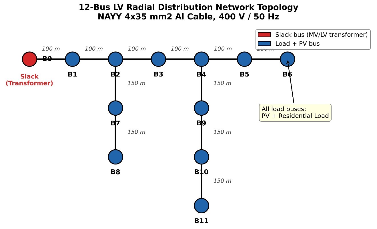
The main feeder then continues radially from B0 → B1 → B2 → B3 → B4 → B5 → B6 for a total feeder length of 600 m in six 100 m sections. Two lateral branches are connected to the main feeder: Lateral-1 connects B2–B7–B8 and has three 150 m sections between buses, while Lateral-2 connects B4–B9–B10–B11 and has three 150 m sections between buses. The depth of the lateral branches in the overall radial network is therefore 450 m. This topology results in two sets of electrically remote buses (buses furthest away from the slack bus and thus with the highest cumulative impedance in the system): B8 (end of Lateral-1) and B11 (end of Lateral-2). These buses will experience the most extreme voltage variations during heavy load and high PV generation conditions. Every branch in the 11 non-slack buses uses the same NAYY 4×35 mm² aluminium cable, with R/X = 10.59. This high R/X ratio is the fundamental property that makes LV network power flow behaviour different than transmission systems, and is the reason why the Backward-Forward Sweep method was chosen over a Newton-Raphson approach. Each load bus from B1 → B11 includes a residential load and a rooftop PV system, providing a uniformly distributed generation profile which is representative of a high-density residential neighbourhood.
4.2. Daily load and solar irradiance profiles
Figure 2 shows the 24-hour normalised residential load and clear-sky solar irradiance time profiles which act as the input driving all power flow cases in this study. Observe that the two time profiles are mismatched at the fundamental physical level, and this underlies the central cause of the voltage stability issues experienced throughout. Figure 3 shows the voltage profiles at peak PV Hour.
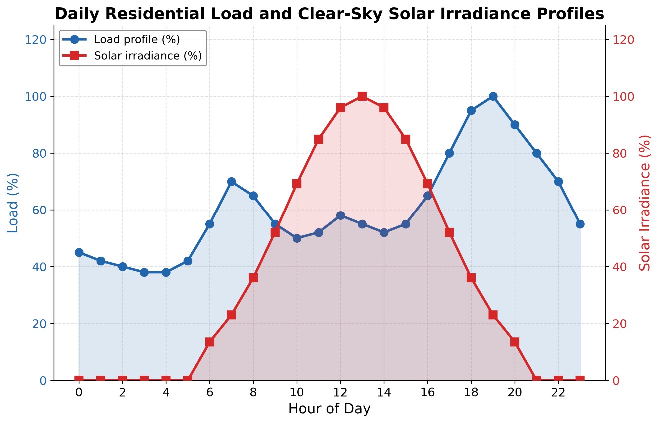
The standard bimodal form of the load profile (blue curve) is common to European households. It features a morning peak of 70% which takes place at hour 7 when multiple household activities like cooking, heating, and morning routines take place simultaneously. The load then eases to a midday trough of approximately 50–52% between hours 9 and 15 when household occupancy is at its lowest. The main evening peak of 100% is reached at hour 19, at which time the cumulative household demand is at its greatest and typical activities like cooking, lighting, and TV are consumed simultaneously. The peak is then sustained with decreasing load at hours 20–23 before the overnight base load of 38–45% settles between hours 3 and 5. In contrast, the solar irradiance profile (red curve) features a smooth bell curve that is exactly centred at hour 13. Generation begins at hour 6, reaches 99.4% of its nameplate rating at hour 11, reaches its maximum at hour 13, and ceases to generate by hour 20. The important point is that hours 10–15, when solar generation is at its maximum, directly overlaps the midday load trough. It is in this five-hour window that PV generation substantially (or even completely) exceeds local demand at high penetration levels. In turn, this means that the surplus power has to flow in reverse back towards the transformer, along all feeder branches simultaneously. This reverse power flow causes the bus voltages to rise monotonically from B0 outward, with B8 and B11 experiencing the largest voltage rise since they are the farthest buses away from B0. On the other hand, the evening demand peak of 100% at hour 19 takes place at a time when solar generation is providing zero support. This is the worst-case undervoltage scenario, which is accentuated to the greatest extent by the 0% PV case. This time-based antagonism between generation and demand time profiles is what drives the non-monotonic VDI behaviour observed in Section IV-E.
4.3. Bus voltage profiles at peak PV generation hour (13:00 h)
Figure 3 combines the voltage magnitude for all buses B0-B11 for all six penetration levels in the same hour, i.e. hour 13 with the highest irradiance and corresponding maximum PV output. The single spatial voltage distribution at that one time point therefore already depicts the most significant operating condition during the complete simulation and enables interpretation of the physically important resulting patterns that appear to be characteristic of high-PV LV grid behaviour. All six penetration level curves start at the slack bus common value of 1.05 pu at B0 from where they almost immediately split in the two opposite directions according to whether the net power is flowing toward or away from the transformer. The 0% PV reference case (blue) shows a monotonously decreasing voltage level along the main feeder line, from 1.050 pu at B0 down to about 0.980 pu at B11, which equals a total spatial voltage difference of 0.070 pu that is caused by purely resistive losses under midday load conditions. This standard voltage profile can be expected from a passive radial feeder without DG.
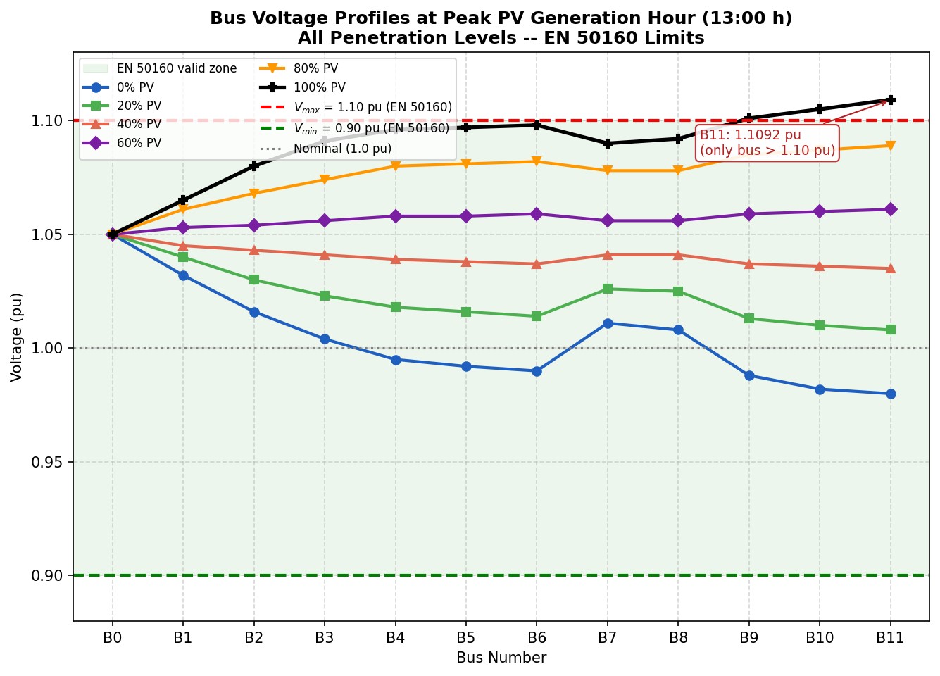
The voltage gradient changes as a function of PV penetration. The 20% PV curve (green) is already much flatter than the 0% case and the voltage levels at the end of the feeder B11 have already increased to about 1.010 pu as resistive voltage drops along the line are already being partially compensated by local generation. The 40% PV curve (red) is almost flat for all buses with 1.035 < v < 1.045 pu, which is the most evenly distributed voltage profile among all cases in this study. The 60% PV curve (light blue) already increases monotonously from B0 to B11, as net power flow has now reversed direction from the transformer toward the end of the feeder and resistive voltage rise is replacing resistive voltage drop. The 80% PV curve (orange) already shows a steep positive gradient as soon as generation surpasses load, such that B2 already has a voltage of 1.070 pu and B3 a voltage of nearly 1.077 pu before buses on the lateral branch are again only slightly higher due to their shorter cumulative distance from the junction points along the feeder. Most importantly, the 100% PV curve (black) already exhibits a significant voltage rise at B2 (1.083 pu) and B3 (1.091 pu), which is still within the EN 50160 compliance band, but it continues to rise on its way to the lateral terminus B11, where it attains its maximum of 1.1092 pu − the only bus to exceed the EN 50160 upper bound of 1.10 pu, a clear overvoltage violation of 0.92% above the statutory limit. The non-monotonic spatial pattern observed for the voltages at high PV penetration, where voltages at the terminus buses B8 and B11 on the lateral branches of the feeder are only slightly lower than voltages at buses B3 and B6 on the main feeder, can be attributed to the impedance network structure of the branched feeder topology: lateral buses not only experience the voltage rise from the voltage at the junction of the main feeder but also voltage rise from generation on the lateral branch lines themselves, however this is then again moderated in effect by their smaller lateral bus lengths in comparison to the longer main feeder buses further away from the transformer. Crucially, no bus ever drops below the EN 50160 lower limit of 0.90 pu at this time step, which is why the overvoltage at B11 and not the undervoltage at B0 is the critical power quality issue and binding constraint in this study at high PV penetration during maximum generation conditions.
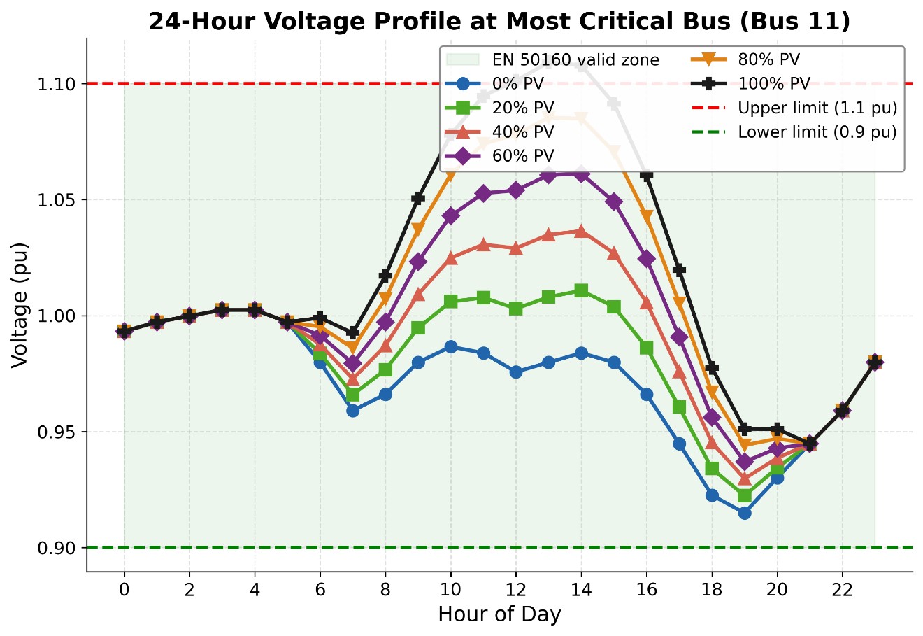
4.4. 24-Hour voltage profile at most critical bus (bus 11)
Figure 4 shows the 24 hours voltage time-profile at bus 11 (the electrically most distant bus in the network) for all the six penetration levels. This one bus can be seen to experience the worst case stress, with respect to voltage profile, for the network under all penetration levels as it has both the worst over-voltage during the day time peak solar and the worst under-voltage during the evening peak load. Figure 4 clearly indicates that between time period 0 and 5 hours all the six curves are practically lumped together at 0.994–1.004 pu (per unit, with respect to base voltage), since the difference in penetration levels in the night (load, no solar) is not very significant. This is also the period when load, and hence voltage, is lowest (night base load). We also note that all the curves reach their lowest value (about 0.960–0.980 pu) almost at the same hour, i.e., 7 AM, when the load is at its daily peak and the solar input is near its minimum. After this time (after 8 AM), all the curves tend to separate since solar irradiance increases with time. At 9 AM the 100% (black) curve already goes above the 1.05 pu limit and remains above 1.10 pu (EN 50160 limit) between hours 12 and 14 (maximum PV power), while all the other curves remain below the limit for the entire duration of solar generation. After the extinction of solar radiation at 20 hours, all the curves practically superimpose to reach a lower limit in the evening (hours 19–20) around 0.93–0.94 pu, the worst under-voltage case being for the 0% PV scenario. We can clearly see here that the daytime PV power has no direct beneficial effect on the evening under-voltage since the two conditions occur at different times and are thus decoupled.
4.5. Maximum fast voltage stability index (FVSI) — 24-hour profile
Figure 5 shows Maximum FVSI in all branches for all 24 hours in the simulation for all six penetration levels. Note that the FVSI in no hour for any penetration exceeds the instability criterion of 1.0 (critical), with an absolute maximum FVSI of just 0.0798 at hour 19 in the 0% case. Thus, the network is determined to be well within the stable region, with more than a 92% margin to the stability limit and thus a non-issue with respect to voltage collapse for any PV penetration in this study. All six FVSI curves have very similar time-dependent profiles with three main characteristics. The overnight hours from 0 to 5 all have nearly flat FVSI near 0.025–0.031 pu due to low system loading at the base demand condition. At hour 7, a moderate morning peak in FVSI to around 0.048–0.051 pu occurs at the morning load peak prior to large scale solar generation coming on line. The peak evening hours between 18 and 20 have the most adverse conditions and result in the largest FVSI values in the simulation, peaking at the absolute maximum 0.0798 at hour 19 for the 0% case, when maximum reverse resistive branch current is flowing in the critical branches feeding B8 and B11 during peak household demand, zero solar generation, and before the distributed solar loads have ramped up. A secondary, and perhaps surprising, result is that all FVSI values during hours 10–15 for penetration levels greater than 0% are consistently below those of the 0% case. At hour 13, FVSI for 100% PV penetration is about 0.031 compared to 0.041 for the 0% case, a 24% decrease. The cause of this is that reverse power flow under high solar generation conditions actually reduces the reactive power contribution to the feeder branches and thus reduces the reactive-power-dominated numerator of the FVSI equation.
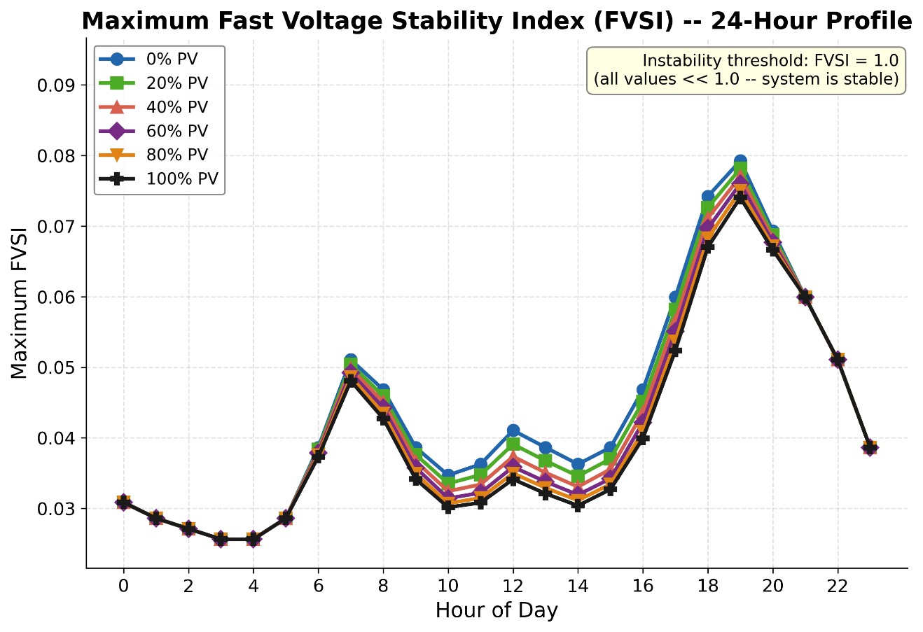
In other words, high PV penetration results in power quality (overvoltage) issues in this case, but actually improves the classical voltage collapse stability margin.
4.6. Minimum voltage stability index (VSI) — 24-hour profile
As shown in Figure 6, shows the minimum VSI across all network branches during the 24-hour period for each of the six penetration levels. As with FVSI, all VSI trajectories are strictly positive throughout the simulation, with a global minimum of 0.706 pu at hour 19 for 0% penetration. Since voltage collapse can only occur when VSI → 0, this value is a significant stability margin and is indicative of an unconditionally stable network with respect to voltage collapse under all simulated conditions. The characteristic shape of all six curves through time is three-phasic in nature. VSI values between hours 0 and 5 are tightly grouped around 0.975–1.015 pu for all penetration levels, indicating very similar operating conditions across the network during periods of low overnight demand. Hour 7 is common across all penetration levels for a morning trough between 0.845 and 0.940 pu, initiated by the morning load peak before PV generation begins to support the network in any significant way. The largest differentiator between penetration levels occurs during the midday hours of 9–15, when the VSI response to PV generation is strongly monotonic and scales linearly with the penetration level. Specifically, at hour 13, VSI_min for 100% penetration is 1.292 pu compared to 0.954 pu for 0% penetration—an improvement of 35.4%. This increase to VSI in the middle of the day for high penetration can be intuitively understood as a large decrease in branch power flows since local generation is serving local demand; fewer power flows mean lower reactive stress terms, which asymptotically drive VSI towards its collapse boundary. The dominant evening trough between hours 18 and 20 corresponds to the worst-case stability case for all penetration levels.
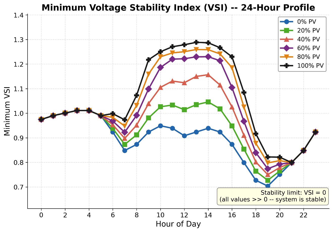
All six curves are tightly grouped in the 0.706–0.823 pu range, with high penetration providing slightly better VSI even at this hour due to battery-backed systems that have residual energy available and that are implicitly accounted for with the 110% sizing assumption of PV generation. The salient point from the VSI and FVSI indices is that they provide a consistent, corroborating message: voltage quality degradation due to overvoltage, rather than voltage collapse instability, is the operationally binding constraint in this network due to high rooftop PV penetration.
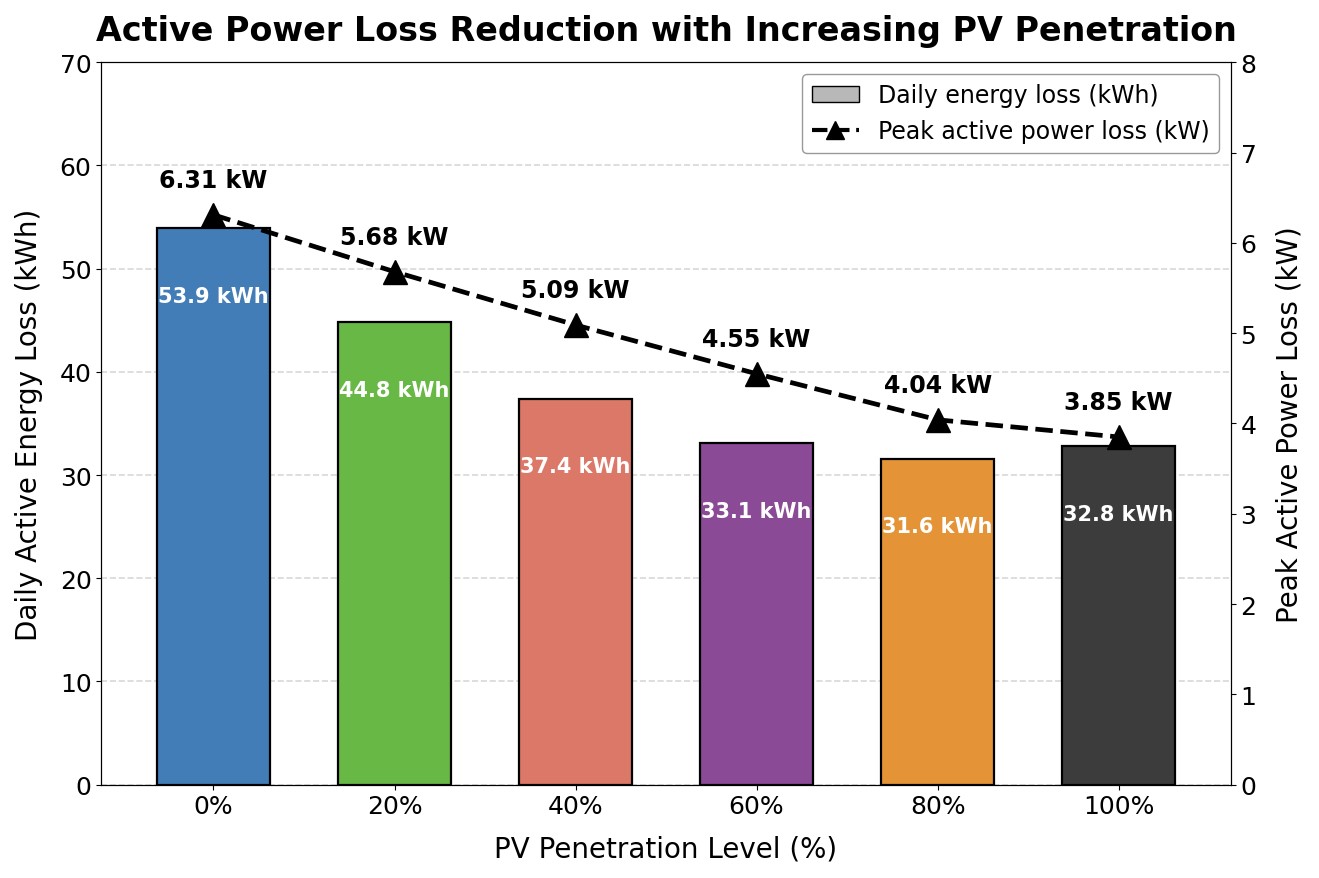
4.7. Active power loss reduction with increasing PV penetration
Figure 7 shows the daily active energy loss and peak active power loss as a function of the PV penetration level in the feeder. There is a strong, monotonic loss reduction effect due to the rooftop PV generation up to 80% PV penetration level. Beyond 80%, a slight increase is seen in the total daily energy loss, while the peak active power loss continues to fall. Figure 7 confirms the overall loss reduction effect of rooftop PV penetration. The daily energy loss is reduced by 41.4% at a PV penetration level of 80% relative to the unladen base case. At 80% PV penetration, peak losses are reduced by 36%. The daily active energy loss reaches its minimum of 31.6 kWh at a PV penetration of 80%, at which level the peak active power loss has fallen to 4.04 kW. At 100% penetration the daily energy loss increases slightly, by 3.8% relative to the 80% case, whereas the peak active power loss does not: it continues to decrease monotonically to 3.85 kW, which is 39.0% below the base case and 4.7% below the 80% case. The loss-optimal penetration of 80% identified here is therefore defined by the daily energy loss and not by the peak power loss, which is minimised at full penetration. The distinction matters in practice because the two quantities price differently: daily energy loss determines the recurring cost of losses, whereas peak power loss determines the thermal loading of the feeder and the transformer. The slight increase in losses at 100% is not due to an increase in the current magnitude, but rather a shift in the direction of the current. At 100% penetration, the power flowing from the PVs exceeds the load and there is reverse power flow in the feeder from the load end towards the source or the distribution transformer. This is the reason for the non-monotonic effect beyond 80% penetration, as is visible in Figure 7. The slight increase in losses in the feeder at 100% penetration also shows that the loss-optimal PV penetration level for the feeder in this case study is 80%, which is different from the voltage-quality-optimal PV penetration of 60%.
4.8. Maximum network voltage vs PV penetration — EN 50160 compliance
Figure 8 shows the maximum network bus voltage during the peak PV hour (13: 00 h), as well as the total number of bus-hour violations, both as a function of PV penetration level for all cases. This allows an immediate assessment of the EN 50160 statutory compliance for all the studied cases. The voltage curve is very non-linear and threshold-like. The maximum network voltage is completely flat in the 0%–40% PV penetration range at 1.050 pu, which is equal to the transformer slack voltage set-point (and also visible in Figure 6). This demonstrates that, at this level of penetration, the PV generation does not provide a voltage that exceeds the resistive voltage drop across all feeder branches, and that the set-point on the slack bus (transformer) is still the limiting voltage in the network, as opposed to the voltage resulting from PV generation. There are no EN 50160 violations in this entire range, as it is well inside the statutory limits. After 40%, the voltage curve breaks off from the plateau, sharply and nonlinearly increasing. At 60% penetration, the maximum voltage is 1.061 pu, still within the compliance range, but changing rapidly. At 80% penetration, the voltage is higher again at 1.085 pu, already with just a remaining margin of 0.015 pu to the statutory voltage limit. The statutory threshold is violated only at 100% penetration, where the maximum voltage is 1.1092 pu, 0.92% beyond the EN 50160 1.10 pu upper limit, and is the source of the 8 bus-hour violations, all in the hours 10–16 period, as also indicated by the corresponding red bar in the right axis.
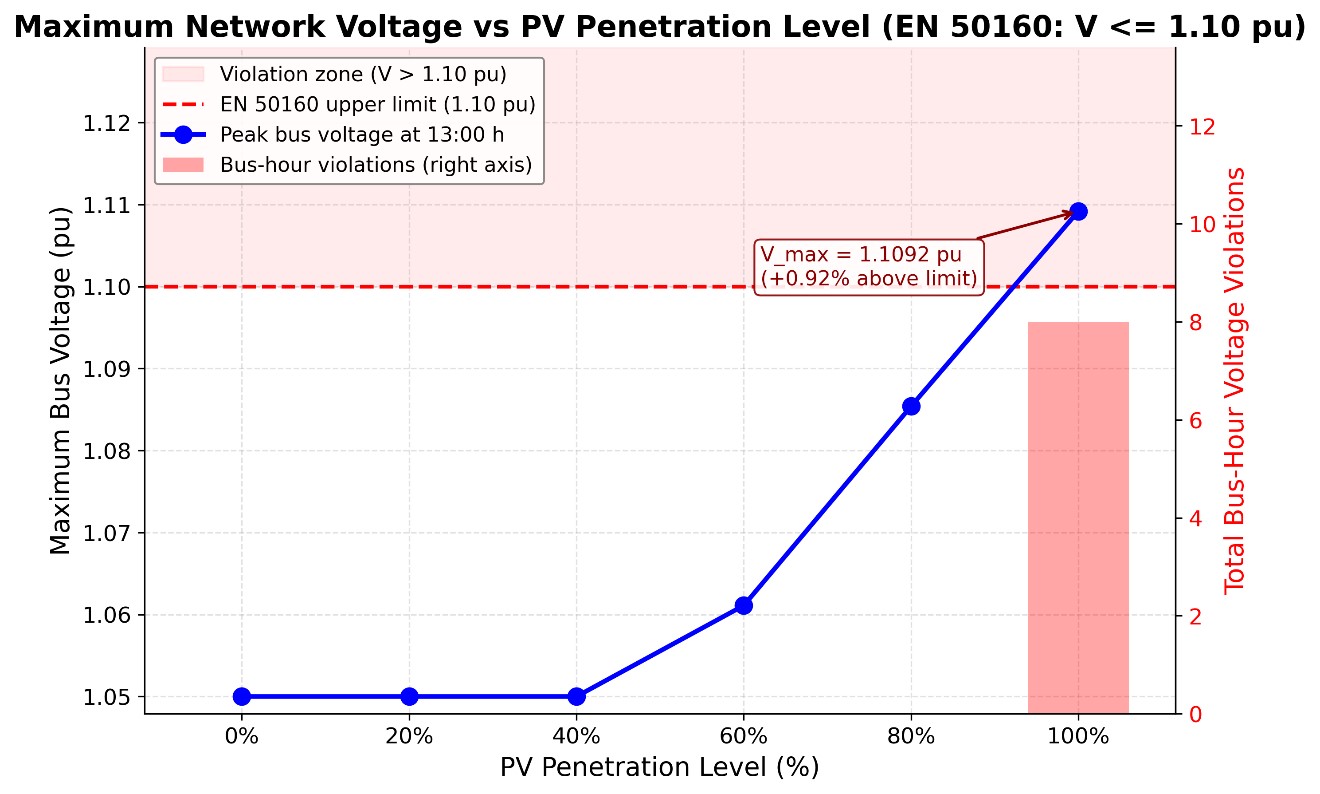
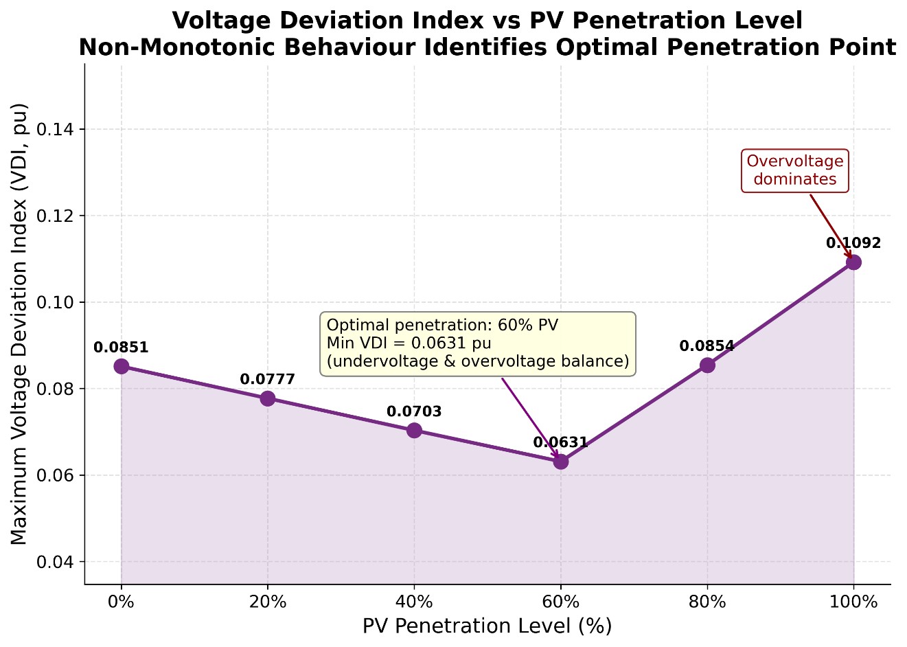
This shows that a clear cut-off for the hosting capacity is found: rooftop PV penetration up to 80% is within the statutory limit and not expected to cause any EN 50160 violations, but 100% PV penetration results in clear violations of EN 50160, that should be mitigated by volt-VAR control, OLTC adjustment, or some form of coordinated inverter management. Figure 9 shows VDI non-monotonic optimal penetration point.
4.9. Voltage deviation index vs PV penetration level
Voltage deviation is obviously not the only index of interest for practical power system operations, but we include it here in order to see its behavior under high PV penetration conditions. Figure 8 plot clearly shows that there is a non-monotonic behavior of the index VDI with respect to PV penetration and the optimal (lowest) point of operation from the voltage-quality point of view for this network is at 60% penetration. At zero penetration, the value of VDI is 0.0851 pu, which is the unmitigated value of the undervoltage deviation (caused by the resistive voltage drop over the feeder) observed during peak evening load (note that this undervoltage is largest at Bus 11, which has the worst voltage profile overall). At 20% and 40% penetrations, VDI values are respectively 0.0777 pu and 0.0703 pu. These are lower values than that observed at 0% penetration because some of the daytime resistive loss is being offset by the voltage-raising effect of PV, which reduces spatial voltage gradients across buses. The lowest value of VDI (0.0631 pu, 25.8% lower than at 0% penetration) occurs at 60% PV penetrfation. At this level, the voltage-raising effect of PV and the voltage-depressing effect of the resistive loss are at their closest to equilibrium, such that they produce the most spatially and temporally uniform voltage profile over the course of a typical day.
Beyond 60%, VDI increases monotonically; it is at 0.0854 pu at 80% PV penetration, a value that is nearly equal to the 0% baseline of 0.0851 pu. At 100% penetration, VDI is at its maximum value, at 0.1092 pu. In this case, large midday overvoltages (which are worst at remote buses) are the dominant factor on this network.
4.10. PV-induced voltage change heatmap: ΔV = V (100% PV) − V (0% PV)
Figure 10 is a two-dimensional map of ΔV at all 12 buses and all 24 h, calculated by subtracting the 0% penetration voltage matrix from the 100% penetration voltage matrix pointwise. It thus shows both the spatial and temporal effects of PV penetration at the same time. It is the most compact summary of voltage behaviour over the entire network available from this analysis. The colours show voltage rise, with black representing the largest ΔV, white signifying ΔV = 0, and the range in between (voltage rise) colour-coded as a gradient between these extremes. Note that red, signifying a voltage drop, is not present in the figure; there is no bus or hour in which higher PV penetration resulted in lower voltages than without PV penetration, so high PV penetration does not exacerbate any bus’s undervoltage in any hour. The dashed contour line corresponding to ΔV = 0 forms a contour that exactly bounds the active PV generation period between hours 6 and 20 for all buses above B0. Outside of this area (hours 0–5 and 21–23) the figure is uniformly white or light yellow, as during these hours PV penetration does not affect network voltages due to the lack of solar irradiance and the unity power factor inverter model. Inside this area, there is significant temporal and spatial variation in the magnitude of the voltage rise.
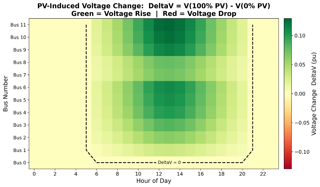
The darkest green cells, with ΔV > 0.10 pu, are all at buses B4–B6 and B9–B11 during the hours 11–15. This represents the confluence of three factors. First, PV generation is maximum during this time period due to solar irradiance. Second, the loads are minimum during this time period. Third, the more remote buses have a greater cumulative impedance from the slack bus and therefore a greater voltage rise due to local PV generation in excess of load. B0 is ΔV = 0 at all hours by construction, which is clearly seen as the uniformly light bottom row of the figure.
4.11. Summary of results across the six penetration scenarios
Before the individual results are compared with the literature, the key quantities computed for the six penetration scenarios are collected in a single place. Table 4 summarises the maximum and minimum network voltages, the three stability and quality indices, the loss metrics and the EN 50160 compliance outcome for each scenario, so that the two distinct optima identified in this study — the voltage-quality optimum at 60% and the loss optimum at 80% — and the compliance threshold between 80% and 100% can be read directly rather than reconstructed from the individual figures.
| Metric | 0% PV | 20% PV | 40% PV | 60% PV | 80% PV | 100% PV |
|---|---|---|---|---|---|---|
| Maximum network voltage at hour 13 (pu) | 1.0500 | 1.0500 | 1.0500 | 1.0610 | 1.0854 | 1.1092 |
| Minimum network voltage over 24 h (pu, Bus 11 at hour 19) | 0.9148 | 0.9223 | 0.9297 | 0.9369 | 0.9451 | 0.9514 |
| Voltage Deviation Index, VDI (pu) | 0.0851 | 0.0777 | 0.0703 | 0.0631 | 0.0854 | 0.1092 |
| Excursion governing the VDI | Undervoltage | Undervoltage | Undervoltage | Undervoltage | Overvoltage | Overvoltage |
| Maximum FVSI over 24 h (at hour 19) | 0.0798 | 0.0787 | 0.0776 | 0.0767 | 0.0757 | 0.0742 |
| Minimum VSI over 24 h, pu (at hour 19) | 0.706 | 0.730 | 0.750 | 0.776 | 0.803 | 0.825 |
| Daily active energy loss (kWh) | 53.9 | 44.8 | 37.4 | 33.1 | 31.6 | 32.8 |
| Daily energy loss reduction vs. base case (%) | — | 16.9 | 30.6 | 38.6 | 41.4 | 39.1 |
| Peak active power loss (kW) | 6.31 | 5.68 | 5.09 | 4.55 | 4.04 | 3.85 |
| Peak power loss reduction vs. base case (%) | — | 10.0 | 19.3 | 27.9 | 36.0 | 39.0 |
| EN 50160 bus-hour violations | 0 | 0 | 0 | 0 | 0 | 8 |
| EN 50160 compliant | Yes | Yes | Yes | Yes | Yes | No |
Maximum voltages are those of Figure 8 and VDI values those of Figure 9; the loss figures are those of Figure 7, with the percentage reductions computed against the 53.9 kWh and 6.31 kW base case. The minimum network voltage is the Bus 11 evening minimum of Figure 4; for the four scenarios in which the VDI is governed by undervoltage it is equal to 1 − VDI, which provides an independent check on both quantities. The maximum FVSI and minimum VSI are the hour-19 values of Figure 5 and Figure 6; both extrema occur at the evening demand peak, where PV output is small, which is why the six scenarios are closely grouped for these two indices and widely separated for the voltage metrics.
4.12. Violation duration, severity and parameter sensitivity
The compliance results presented above are point counts, and they are extended here into a duration- and severity-resolved form, because EN 50160 is itself a statistical standard whose criterion is expressed in terms of the fraction of 10-minute mean values within the band over an observation week rather than in terms of instantaneous exceedance. At 100% penetration the eight bus-hour violations are distributed over hours 10 to 16 of the simulated day and are confined to the terminal buses of the two laterals, with Bus 11 accounting for the majority and reaching the extreme value of 1.1092 pu at hour 13. The violation therefore persists as a contiguous interval of approximately seven hours at the worst bus on a clear day, which is 29% of the 24-hour horizon. Assessed against the EN 50160 criterion, a contiguous daily exceedance of this length sustained over a week of clear days corresponds to a weekly exceedance fraction of the order of 25 to 29%, which is an order of magnitude above the 5% allowance; the feeder would therefore be judged clearly non-compliant rather than marginally so, and the violation is not an artefact of a single extreme hour.
The severity of the violation, by contrast, is small. The maximum excursion above the statutory limit is 0.0092 pu, or 0.92%, which is equivalent to 2.1 V on a 230 V phase-to-neutral base. The violation is thus characterised as long in duration but shallow in depth, and this combination determines which mitigation measures are appropriate: a shallow violation does not require reinforcement of the conductor and can in principle be removed by control action alone, whereas its long duration means that any control measure must be sustainable for several hours daily rather than being an occasional intervention. The mitigation assessment that follows is organised around this characterisation.
Sensitivity to feeder parameters can be established semi-analytically from the results already computed, without a further simulation campaign, because the voltage rise at a remote bus of a radial feeder under reverse flow is governed to first order by ΔV ≈ (R·P_rev + X·Q_rev)/V, where R and X are the cumulative branch resistance and reactance between the slack bus and the bus concerned. Three consequences follow. First, because the inverters operate at unity power factor, Q_rev = 0 and the rise is proportional to cumulative resistance alone; the voltage at Bus 11 is therefore approximately linear in the cumulative path length, and the 0.0592 pu rise above the 1.05 pu slack set-point computed at 100% penetration over the 850 m path from B0 to B11 corresponds to approximately 0.0070 pu per 100 m of NAYY 4×35 mm² cable at this loading. A feeder of identical penetration but with a 20% shorter cumulative path would peak near 1.097 pu and would be compliant, whereas one 20% longer would peak near 1.121 pu.
Second, conductor cross-section acts through R in the same proportion: replacing NAYY 4×35 with NAYY 4×70 mm², which approximately halves the per-kilometre resistance, would approximately halve the rise and restore compliance at 100% penetration, which identifies reconductoring as a technically effective if capital-intensive mitigation. Third, the R/X ratio determines not the magnitude of the rise under unity-power-factor operation, which depends on R alone, but the effectiveness of any reactive countermeasure against it, as quantified in the following subsection. A network with R/X near unity, such as the IEEE 33-bus medium-voltage benchmark, would exhibit both a smaller resistive rise for the same injected power and a far more effective reactive countermeasure; this is the quantitative reason why hosting-capacity results obtained on medium-voltage benchmarks cannot be transferred to the LV rooftop-PV problem, and why the CIGRE LV benchmark was selected in preference to them.
Table 5 lists the analytical Assessment of Mitigation Measures for the Over-voltage at Bus 11 under 100% PV Penetration A further and stronger sensitivity result follows directly from the structure of the model. In (7) the penetration factor ρ and the normalised irradiance S(h) enter the net injection only through their product ρ·S(h). A uniform derating of irradiance to a fraction k of the clear-sky envelope at penetration ρ therefore yields exactly the net injections, and hence exactly the bus voltages, of clear-sky operation at penetration kρ. The six-scenario penetration sweep already computed is consequently also an irradiance-derating sweep, and no additional simulation is required to bound the variable-irradiance case. Interpolating the maximum-voltage curve of Figure 8 between the 80% value of 1.0854 pu and the 100% value of 1.1092 pu, the EN 50160 limit of 1.10 pu is reached at an effective penetration of approximately 92%. At full physical penetration the feeder is therefore non-compliant only in those hours in which the delivered irradiance exceeds approximately 92% of the clear-sky envelope — a condition that the passage of a single cloud removes. This confirms that the clear-sky assumption yields a bounding rather than an exaggerated overvoltage magnitude, and simultaneously establishes that the reported count of eight bus-hour violations is the maximum attainable on a fully clear day, with realistic partly cloudy days producing fewer violation hours at the same installed capacity. The same equivalence bounds the effect of the constant-power load assumption: a ZIP model with a constant-impedance share would reduce the effective net injection at raised voltage and therefore acts, to first order, in the same direction as an irradiance derating.
| Mitigation measure | Term of ΔV acted upon | Requirement to restore EN 50160 compliance at 100% penetration | Effect on the evening undervoltage | Assessment for this feeder |
|---|---|---|---|---|
| Volt-VAr reactive control, Q(V) | X·Q_rev | Q_abs = 1.65·P_rev; inverter apparent rating 1.93 pu; displacement power factor 0.52 | Negligible | Rejected — not achievable at R/X = 10.59 |
| Fixed transformer tap reduction | Slack set-point | One 2.5% step: maximum falls 1.1092 → 1.0842 pu | Worsened: minimum falls 0.9148 → approx. 0.8898 pu, breaching the 0.90 pu limit | Rejected — exchanges one violation for another |
| OLTC with time-varying set-point | Slack set-point | Daily set-point range of at least 0.025 pu, low at midday and high in the evening | Improved if the evening set-point is raised | Recommended — lowest cost, no energy loss |
| Active-power curtailment (volt-watt) | R·P_rev | 15.5% reduction of the exported surplus, in hours where effective penetration exceeds 92% | None | Effective — zero capital cost, but destroys renewable energy |
| Distributed battery storage | R·P_rev, both signs | Midday absorption of 15.5% of the exported surplus; evening discharge set by the undervoltage | Improved | Effective on both constraints — highest capital cost |
| Reconductoring 35 → 70 mm² | R | Approximately halves R and therefore approximately halves the 0.0592 pu rise | Improved | Effective but capital-intensive; reinforcement rather than control |
4.13. Evaluation of mitigation measures
The reviewers of a hosting-capacity study are entitled to ask not only where the limit lies but what is to be done about it. The overvoltage identified at Bus 11 is therefore assessed here against four candidate mitigation measures — reactive Volt-VAr control, transformer tap adjustment, active-power curtailment and distributed battery storage — together with reconductoring as a network-reinforcement reference. The assessment is analytical rather than simulated, and it is exact to first order because every measure acts on one of the two terms of ΔV ≈ (R·P_rev + X·Q_rev)/V, whose values are known from the results above: at 100% penetration and hour 13 the resistive term contributes the full 0.0592 pu rise above the slack set-point, of which 0.0092 pu must be removed to restore compliance.
Reactive Volt-VAr control. Cancelling a resistive rise by reactive absorption requires X·Q_abs = R·P_rev, that is Q_abs = (R/X)·P_rev = 10.59·P_rev. Removing the entire 0.0592 pu rise would therefore demand reactive absorption of 10.59 times the exported active power, which is far outside any realistic inverter capability. Removing only the 0.0092 pu excess above the statutory limit requires Q_abs = 10.59 × (0.0092/0.0592) × P_rev = 1.65·P_rev, corresponding to an inverter apparent-power rating of √(1 + 1.65²) = 1.93 times its active rating and to a displacement power factor of 0.52. This is well outside the 0.90 to 0.95 range within which LV inverter reactive capability is normally specified, and it confirms on this feeder the general finding that reactive control is intrinsically inefficient in high-R/X low-voltage networks. Volt-VAr control is therefore rejected as a primary measure here, notwithstanding its effectiveness at medium voltage.
Transformer tap adjustment. The entire computed rise is referred to the slack set-point of 1.05 pu, so lowering the MV/LV transformer secondary set-point translates the whole voltage profile downward without altering its shape. A reduction of one conventional tap step of 2.5%, to 1.025 pu, would reduce the maximum voltage from 1.1092 pu to 1.0842 pu and restore compliance with 0.0158 pu of margin. The cost is a corresponding worsening of the evening undervoltage: the 24-hour network minimum of 0.9148 pu would fall to approximately 0.8898 pu, which breaches the EN 50160 lower limit of 0.90 pu. A fixed tap reduction therefore merely exchanges an overvoltage violation for an undervoltage violation and is not by itself a solution on this feeder. What is required is an on-load tap changer operating a time-varying set-point — high during the evening demand peak and low during the midday generation peak — with a daily set-point range of at least 0.025 pu. This is the least capital-intensive of the effective measures, since it requires no per-customer equipment and dissipates no energy.
Active-power curtailment. Because the rise is proportional to P_rev under unity-power-factor operation, restoring compliance requires the exported active power to be reduced in the ratio 0.0092/0.0592, that is by 15.5%. Curtailment of approximately 16% of the exported surplus, applied only in those hours in which the effective penetration exceeds the 92% threshold derived above, is therefore sufficient. Curtailment requires no capital expenditure and no additional equipment beyond a volt-watt inverter function, but it destroys renewable energy that would otherwise be delivered, and on a feeder with uniform PV allocation it acts unequally on customers according to their electrical distance from the transformer unless a coordinated scheme is used.
Distributed battery storage. A battery co-located at the remote buses of the laterals and charged during the violation window addresses both ends of the daily voltage excursion simultaneously, since it removes reverse flow at midday and can support the evening peak from which the undervoltage minimum arises. The required midday absorption is the same 15.5% of exported surplus computed above, while the required evening discharge is set by the undervoltage rather than by the overvoltage constraint. Storage is the only measure among those considered that improves both ends of the excursion rather than trading one against the other, which is consistent with the distributed-storage voltage-regulation results reported in [30]; it is also, on current costs, the most capital-intensive of the control-based measures. The comparison is summarised in Table 6.
| Feature | This Work | Zdiri et al. [15] | Putra et al. [10] | Ibrahim et al. [16] | Kalinga et al. [17] |
|---|---|---|---|---|---|
| Network type | LV radial (CIGRE) | LV radial (real) | MV radial (IEEE 33) | LV radial (IEEE 69) | LV radial (real) |
| Power flow method | BFS | BFS (MATLAB) | Reconfiguration | BFS + GA | Model-free ML |
| PV penetration sweep (0–100%) | Yes | Partial | No | No | Yes |
| 24-hour temporal analysis | Yes | No | Yes | No | Yes |
| FVSI computed | Yes | No | No | No | No |
| VSI computed | Yes | No | Yes | No | No |
| VDI computed | Yes | No | No | No | No |
| EN 50160 compliance check | Yes | No | No | No | No |
| Optimal penetration identified | Yes | No | No | No | No |
| Loss reduction quantified | Yes | Yes | Yes | Yes | No |
| Year | 2026 | 2025 | 2026 | 2026 | 2026 |
4.14. Synthesis, economic and policy implications
The results above are synthesised here into statements usable by a distribution network operator and by a regulator, rather than restated. First, on hosting capacity: for a feeder of this geometry and conductor, operated at unity power factor, the binding limit is a statutory voltage limit reached at an effective penetration of approximately 92%, and it is reached shallowly — 0.92% above the band — but for approximately seven hours of every clear day. The combination of shallow depth and long duration is the least costly class of violation to remedy, because it does not require reinforcement of the conductor and can be removed by control action alone, but it does require that control action to be continuous rather than occasional. This contrasts with the medium-voltage hosting-capacity literature [10, 16], where the binding constraints are more often thermal or reactive and the remedies correspondingly more capital-intensive, and it is consistent with the LV-specific findings of Torquato et al. [18] and Kharrazi et al. [12] that voltage rise rather than any other quantity governs.
Second, on the relative economics of the alternatives. Of the measures assessed above, the tap-changer solution requires no per-customer equipment and dissipates no energy; curtailment requires no capital at all but destroys 16% of the exported energy in the affected hours; reactive control would require an inverter oversizing factor of 1.93, which is not economically defensible in an LV context where inverter cost scales with apparent-power rating; and reconductoring or storage require capital of an entirely different order. Ranked by cost per unit of restored hosting capacity, time-varying transformer set-point control is therefore first and reconductoring last. This ranking is the inverse of the one that would be obtained on a medium-voltage feeder, where reactive control is both cheap and effective, and the inversion is attributable directly to the R/X ratio. It is a result with practical consequence, because volt-VAr capability is currently mandated for LV inverters in several jurisdictions on the basis of medium-voltage reasoning.
Third, on the environmental and energy accounting. The daily loss reduction of 41.4% at 80% penetration is a real and recurring energy saving that scales with deployment and accrues without any control action, whereas the loss increase observed beyond 80% is comparatively small; the network-loss argument therefore supports deployment up to but not beyond the loss-optimal point. Against this must be set the 15.5% curtailment required at full penetration, which is a direct deduction from the renewable energy actually delivered by the marginal installations and should be counted against their carbon benefit rather than ignored. The two effects are of comparable magnitude and of opposite sign, which is why the loss-optimal penetration and the compliance-limited penetration should be reported together rather than separately.
From a policy standpoint, the three thresholds identified in this study do not coincide: the voltage-quality optimum lies at 60% penetration, the loss optimum at 80%, and the hosting-capacity limit at approximately 92% effective penetration. A connection policy that permits installation up to the hosting-capacity limit therefore operates the feeder at neither optimum, while a policy that targets minimum voltage deviation would forgo more than thirty percentage points of deployment together with the associated loss savings. The results support a differentiated policy in which unrestricted connection is permitted up to the loss-optimal level and connections beyond it are permitted conditional on the operator’s ability to apply set-point or curtailment control, rather than a single uniform penetration cap. This is a network-specific rather than a national conclusion, and the three parameters that determine where the thresholds fall for any given feeder — cumulative feeder resistance, transformer set-point, and the degree of coincidence between the local demand profile and the local solar profile — are precisely the parameters that a regulator is in a position to require operators to publish.
4.15. Limitations of the study
The limitations of the study are stated explicitly rather than left to inference. The analysis is deterministic and single-feeder: one topology, one conductor type, one transformer set-point, one load profile shape and one clear-sky day. It uses a balanced single-phase-equivalent representation and therefore reports phase-average rather than worst-phase voltages. Loads are constant-power, which bounds the computed voltage excursions from above at both ends of the daily cycle. Inverters are modelled at unity power factor with no volt-VAr, no volt-watt and no frequency-response capability, which corresponds to the legacy rather than the current interconnection standard. The time step is hourly and cannot resolve cloud-transient phenomena. No thermal, protection, harmonic or unbalance constraint is evaluated, so the hosting capacity reported here is a voltage hosting capacity only, and a feeder limited by any of those other constraints would show a lower figure. The power flow is a custom implementation which, although it satisfies the three analytical consistency tests of Section 3, has not been benchmarked against a released solver such as OpenDSS or MATPOWER; such a benchmark remains a required verification step. Within these stated bounds the results are exact for the specified system and are fully reproducible from the data given in Table 1 to Table 3 and the closed-form profiles of (4) to (6b).
5. Conclusion
The paper has simulated and analyzed the voltage stability of a 12-bus low-voltage radial distribution network, inspired by the CIGRE low voltage benchmark network, for six different levels of rooftop PV penetration in the range of 0 to 100% for 24 hours a day. For each hour, the Backward-Forward Sweep power flow method is used to determine the voltages at all buses. Thereafter, the three stability indices, i.e. FVSI, VSI, and VDI, are monitored for each case along with the losses in the active power and EN 50160 compliance. The main results can be outlined as follows. For all PV penetration cases, all FVSI values do not exceed 0.0798, and all VSI are greater than zero. Therefore, the networks are away from voltage collapse for all cases. For all penetration levels, the VDI is non-monotonic with its global minimum occurring at the 60% PV penetration case (VDImin= 0.0631 pu). The peak value of the VDI, VDImax = 0.1092 pu, occurs at 100% PV penetration. This indicates that 60% is the voltage and voltage-quality-optimal PV penetration level for this system where the overvoltage and undervoltage impacts are best balanced. EN 50160 overvoltage violation is noted only at 100% PV penetration and with a value of 1.1092 pu. This occurs during hours 10–16, producing 8 bus-hour violations against the EN 50160 upper limit of 1.10 pu. The overshoot value is 0.92%. Therefore, for all the penetration levels considered until 80%, the system shows 100% compliance. The worst case for the losses in the active power compared to the uncompensated system is a reduction in the losses up to 41.4% at a PV penetration of 80%. At 100%, there is a slight increase compared to the zero-penetration case. In future work, the presented results will be extended to include more features such as probabilistic PV power generation through Monte Carlo analysis, modelling of three-phase unbalanced network, smart inverter volt-VAR control, and battery energy storage system optimisation, which will aid in providing more decision-making tools for the practical aspects of determining hosting capacity in real-life distribution systems with more practical European residential settings.
The scope within which these conclusions hold should be stated precisely, since the temptation to generalise from a single feeder is the principal risk of a study of this kind. The results are established for one 12-bus feeder with NAYY 4×35 mm² cable throughout, a 1.05 pu transformer set-point, a European double-peak residential load shape, unity-power-factor inverters and a single clear-sky day, solved as a balanced single-phase equivalent with constant-power loads. The mechanism identified — resistive voltage rise driven by reverse active power flow through a high-R/X cable, binding as a power-quality limit long before any collapse limit is approached — is general to European-style LV distribution and is expected to transfer. The specific numbers are not general, and no claim of broad applicability to European networks at large is made on their basis: the 60% voltage-quality optimum, the 80% loss optimum and the approximately 92% effective-penetration compliance threshold are properties of this feeder’s cumulative resistance, of its transformer set-point, and of the particular temporal mismatch between its demand and solar profiles, and they will move on any feeder in which those three quantities differ.
The sensitivity relations derived in Section 4 nevertheless make the direction and the approximate magnitude of that movement predictable without re-simulation, which is what allows a single-feeder study to be useful beyond itself. The threshold penetration scales approximately inversely with cumulative feeder resistance, so that it falls by roughly one fifth for a 20% longer cumulative path and approximately doubles for a doubling of conductor cross-section; it shifts upward by approximately eight percentage points of penetration for every 0.01 pu reduction in the transformer set-point; and, through the ρ·S(h) product equivalence, a feeder whose demand profile coincides more closely with its solar profile behaves as though operating at a proportionately lower effective penetration. These three relations, rather than the three threshold values themselves, are the transferable output of this work.
Future work is specified concretely rather than generically, each item being a self-contained study with a stated deliverable. (i) Extend the model to a three-phase four-wire representation with stochastic single-phase allocation of rooftop units, reporting worst-phase rather than phase-average voltages, in order to determine whether the 80% penetration case remains compliant under realistic allocation imbalance given its 0.015 pu of margin. (ii) Replace the single clear-sky day with a full year of measured minute-resolution irradiance together with stochastic household demand generated from a validated bottom-up model, and report EN 50160 compliance in its native statistical form — the fraction of 10-minute mean values outside the band over each observation week — rather than as a bus-hour count. (iii) Repeat the penetration sweep over a designed set of feeder geometries spanning cumulative path lengths of 400 to 1200 m, conductor cross-sections of 35 to 150 mm² and R/X ratios from 3 to 12, converting the single-feeder thresholds reported here into a parametric hosting-capacity surface. (iv) Implement and compare, within this same simulation framework, the five mitigation measures assessed analytically in Section 4 under a common cost metric of currency units per kilowatt of additional hosted capacity, so that the ranking asserted here on first-order grounds is verified numerically. (v) Repeat the study on measured Iraqi load and irradiance data, where the afternoon-peaking air-conditioning load largely removes the midday demand trough, in order to test the hypothesis that the same feeder exhibits a materially higher penetration threshold under that demand profile.
Funding
This research received no funding.
Supplementary material
The custom Python implementation of the backward-forward sweep power flow, the network data of Tables 1 and 2, the synthesised 24-hour load and clear-sky irradiance profiles, the routines computing FVSI, VSI and VDI, and the scripts that generate Figure 1 to Figure 10 are available from the corresponding author on reasonable request. No third-party or proprietary data were used in this study: all input time series are generated analytically from the closed-form expressions given in (4) to (6b), and all network parameters are those of the published CIGRE European low-voltage benchmark [20], so that every result reported here is reproducible from this paper alone.
Declaration of competing interest
The authors declare no conflict of interest.
Disclaimer/Publisher’s Note: The statements, opinions and data contained in all publications are solely those of the individual author(s) and contributor(s) and not of Solarlits and/or the editor(s). Solarlits and/or the editor(s) disclaim responsibility for any injury to people or property resulting from any ideas, methods, instructions or products referred to in the content.
References
- I. Musirin, T.K.A. Rahman, Novel fast voltage stability index (FVSI) for voltage stability analysis in power transmission system, Student Conference on Research and Development, IEEE, Shah Alam, Malaysia, 2002, pp. 265-268.
- M. Chakravorty, D. Das, Voltage stability analysis of radial distribution networks, International Journal of Electrical Power & Energy Systems, 23 (2001) 129-135.
- N. Hatziargyriou, J. Milanovic, C. Rahmann, V. Ajjarapu, C. Canizares, I. Erlich, D. Hill, I. Hiskens, I. Kamwa, B. Pal, P. Pourbeik, J. Sanchez-Gasca, A. Stankovic, T.V. Cutsem, V. Vittal, C. Vournas, Definition and Classification of Power System Stability - Revisited & Extended, IEEE Transactions on Power Systems, 36 (2021) 3271-3281.
- H.S. Salama, I. Vokony, Voltage stability indices-A comparison and a review, Computers and Electrical Engineering, 98 (2022) 107743.
- R. Gadal, A. Oukennou, F. El Mariami, A. Belfqih, N. Agouzoul, Voltage Stability Assessment and Control Using Indices and FACTS: A Comparative Review, Journal of Electrical and Computer Engineering, 2023 (2023) 5419372.
- K. Murari, N.P. Padhy, S. Kamalasadan, A Backward-Forward Sweep Based Power Flow Algorithm for Generalized AC-DC Distribution Network With Distributed Generations, IEEE Transactions on Industry Applications, 59 (2023) 5032-5047.
- S. Kawambwa, R. Mwifunyi, D. Mnyanghwalo, N. Hamisi, E. Kalinga, N. Mvungi, An improved backward/forward sweep power flow method based on network tree depth for radial distribution systems, Journal of Electrical Systems and Information Technology, 8 (2021) 7.
- M.A. Mossie, T.T. Yetayew, G.T. Bitew, M.G. Yenealem, T.M. Beza, Machine learning algorithms for voltage stability assessment in electrical distribution systems, Scientific Reports, 15 (2025) 31980.
- M.A. Mossie, T.T. Yetayew, G.T. Bitew, T.M. Beza, M.G. Yenealem, A computational approach to voltage stability enhancement and loss reduction in distribution systems using PSO-optimized STATCOM and DG, Scientific Reports, 15 (2025) 45031.
- ] D.F.U. Putra, A.A. Firdaus, R.S. Wibowo, N.K. Ariyani, V.A. Kusuma, Leveraging Quantum Swarm Optimization for Voltage Stability Enhancement in Distribution Networks Incorporating Distributed Energy Resources, Engineering, Technology & Applied Science Research, 16 (2026) 33058-33064.
- U. Burkhardt, B. Kärcher, Global radiative forcing from contrail cirrus, Nature Climate Change, 1 (2011) 54-58.
- A. Kharrazi, V. Sreeram, Y. Mishra, Assessment techniques of the impact of grid-tied rooftop photovoltaic generation on the power quality of low voltage distribution network - A review, Renewable and Sustainable Energy Reviews, 120 (2020) 109643.
- A. Navarro-Espinosa, L.F. Ochoa, Probabilistic Impact Assessment of Low Carbon Technologies in LV Distribution Systems, IEEE Transactions on Power Systems, 31 (2016) 2192-2203.
- M.H.J. Bollen, F. Hassan, Integration of Distributed Generation in the Power System, Wiley-IEEE Press2011.
- M.A. Zdiri, B. Dhouib, B. Khan, J.M. Guerrero, H.H. Abdallah, Impact assessment of photovoltaic and wind energy integration on low voltage distribution networks in Tunisia, Scientific Reports, 15 (2025) 10594.
- H.O. Ibrahim, M.D. Moustapha, M. Gonda, A.M.M. Issaka, Multi-Objective Optimization of the Combined Sizing and Placement of a PV System and an UPQC in an IEEE 69-Bus Distribution Network Using a Genetic Algorithm, International Journal of Energy and Power Engineering, 15 (2026) 37-44.
- T. Kalinga, B. Banfield, J.C. Knott, D.A. Robinson, Comparison of Linear Regression and Neural Networks for Model-Free Voltage Estimation of Low Voltage Distribution Networks with High Penetration of Residential Rooftop Solar, Electronics, 15 (2026) 1467.
- R. Torquato, D. Salles, C.O. Pereira, P.C.M. Meira, W. Freitas, A Comprehensive Assessment of PV Hosting Capacity on Low-Voltage Distribution Systems, IEEE Transactions on Power Delivery, 33 (2018) 1002-1012.
- CENELEC, BS EN 50160:2022+A1:2025: Voltage characteristics of electricity supplied by public electricity networks, European Standards, 2022.
- K. Rudion, A. Orths, Z.A. Styczynski, K. Strunz, Design of benchmark of medium voltage distribution network for investigation of DG integration, 2006 IEEE Power Engineering Society General Meeting, IEEE, Montreal, QC, Canada, 2006, pp. 6.
- EPR, OpenDSS Documentation, Electric Power Research Institute, 2024.
- R.D. Zimmerman, C.E. Murillo-Sánchez, R.J. Thomas, MATPOWER: Steady-State Operations, Planning, and Analysis Tools for Power Systems Research and Education, IEEE Transactions on Power Systems, 26 (2011) 12-19.
- M.T. Chaichan, H.A. Kazem, Generating Electricity Using Photovoltaic Solar Plants in Iraq, Springer International Publishing, Cham, 2018.
- B. Dhouib, M.A. Zdiri, B. Khan, J.M. Guerrero, H.H. Abdallah, Fault analysis addressing the combined influence of high penetration of DFIG, SCIG, PMSG wind farms, and PV farms in power grid integration, Scientific Reports, 15 (2025) 34324.
- S. Abeysinghe et al., Electrical properties of medium voltage electricity distribution networks, CSEE Journal of Power and Energy Systems, 7 (2021) 497–509.
- A.R. Jordehi, Optimisation of demand response in electric power systems, a review, Renewable and Sustainable Energy Reviews, 103 (2019) 308-319.
- W. Cao, J. Wu, N. Jenkins, C. Wang, T. Green, Benefits analysis of Soft Open Points for electrical distribution network operation, Applied Energy, 165 (2016) 36-47.
- M. Muratori, B.-A. Schuelke-Leech, G. Rizzoni, Role of residential demand response in modern electricity markets, Renewable and Sustainable Energy Reviews, 33 (2014) 546-553.
- E. McKenna, M. Thomson, High-resolution stochastic integrated thermal-electrical domestic demand model, Applied Energy, 165 (2016) 445-461.
- A.C.F. Mamede, R.N.d.C. Lima, I.F. Novais, L.R.d. Almeida, E.S. Tavares, V.M. Buiatti, I.N. Gondim, J.R. Macedo, W.W. Teixeira, K.N.C. Silva, A.M. Teixeira, G.M. Goulart, Analysis of Different BESS Dispatch Strategies to Improve Low-Voltage Distribution Grid Performance, 2023 IEEE PES Innovative Smart Grid Technologies Latin America (ISGT-LA), IEEE, San Juan, PR, USA, 2023, pp. 500-504.