

Alaa Alaidroos1,*, Diana Mardenli2
Author affiliations
- 1Architectural Engineering Department, Faculty of Engineering-Rabigh Branch, King Abdulaziz University, Jeddah 21589, Kingdom of Saudi Arabia
- 2Architecture Department, Dar Al Hekma University, Jeddah, Kingdom of Saudi Arabia
*Corresponding author.
- aalaidroos@kau.edu.sa (A. Alaidroos)
- dhmardenli@dah.edu.sa (D. Mardenli)
History: Received 1 August 2026 | Revised 22 August 2026 | Accepted 16 September 2026 | Published online 20 November 2026
Copyright: © 2026 The Author(s). Licensee Solarlits Limited (Hong Kong). This is an open access article distributed under the terms and conditions of the Creative Commons Attribution 4.0 License.
Citation: Alaa Alaidroos, Diana Mardenli, Climate Dependence of the Cooling Energy, Circadian Lighting Trade-off in Dynamically Controlled Hospital Glazing and Shading: A Three-Climate Study, Journal of Daylighting, 13:2 (2026) 793-808. doi: 10.15627/jd.2026.42
Abstract
Dynamic control of window visible transmittance (VT) and shading can simultaneously manage cooling energy demand and circadian effective daylight (Equivalent Melanopic Lux, EML), but whether the resulting trade-off is climate invariant remains untested. This study applies an hourly, EnergyPlus and MATLAB weighted multi-objective control framework to minimize a performance index over visible transmittance and shading projection depth, identically for three climatically distinct hospital sites: Jeddah (hot arid, cooling dominated), Athens (Mediterranean, mixed load), and Seattle (marine, heating leaning). Varying the cooling energy weight WCE throughout its full range (0 to 1) reveals a strongly non-linear trade-off in all three climates, in which circadian performance remains near its limit while nearly all achievable cooling energy savings are obtained, collapsing only when illuminance is given zero weight. The magnitude of achievable cooling energy reduction before this collapse scales inversely with cooling dominance, 5% in Jeddah, 17% in Athens, and 55% in Seattle in relative terms, and only Jeddah shows interior curvature, indicating that a continuously tunable trade-off exists only where cooling load is substantial, while Athens and Seattle behave in a near binary manner. Measured against a static reference, none of the 40 fixed VT and shading configurations reaches the combination of cooling energy and EML delivered by the dynamic control in any of the three climates. Annual control deployment mirrors the same gradient, with an annual mean shading projection of 0.67 m in Jeddah, 0.56 m in Athens, and 0.25 m in Seattle, and in every climate the controller withdraws shading during daylit hours and deploys it when daylight is unavailable. A glare weighted variant of the objective produces the most climate independent result, since prioritizing glare control above a weight of approximately 0.5 to 0.6 collapses mean EML below the WELL Building Standard threshold of 200 EML in all three climates. These findings indicate that the energy circadian trade-off previously identified in hot arid climates is not a general property of dynamic envelope control but is itself climate dependent in both magnitude and shape, with direct implications for how such control strategies should be tuned and implemented in different locations.
Keywords
Circadian lighting, Equivalent melanopic lux, dynamic glazing, Cooling energy, Hospital daylighting, Shading control
Nomenclature
| VT | Visible transmittance of glazing |
| EML | Equivalent Melanopic Lux |
| GI | Daylight glare index (Hopkinson DGI), dimensionless |
| Z | Weighted multi-objective performance index |
| CE | Min-max normalized cooling energy term |
| ill | Min-max normalized illuminance term |
| WCE | Weight coefficient applied to cooling energy |
| Will | Weight coefficient applied to illuminance |
| WGI | Weight coefficient applied to Glare Index |
| IDF | EnergyPlus Input Data File |
| WELL | WELL Building Standard |
| IES | Illuminating Engineering Society |
| Lw | Average luminance of the window seen from the reference point |
| Lb | Background luminance |
| Ω | Solid angle subtended by the window, modified by the Guth position index |
| ω | Solid angle subtended by the window at the reference point |
1. Introduction
Daylight entering a building is no longer treated only as a source of illumination, it is also a circadian input that regulates the human sleep wake cycle through intrinsically photosensitive retinal ganglion cells (ipRGCs), which respond to the intensity, spectrum, and timing of light reaching the eye [1]. This dual role has moved circadian effective metrics into building design guidance and standards practice. The WELL Building Standard sets a daytime Equivalent Melanopic Lux (EML) threshold of 200 for occupied spaces [2], and the CIE S 026/E:2018 standard provides the metrology basis for ipRGC influenced lighting design [3]. Practical targets for daytime, evening, and nighttime light exposure have been published to translate this physiology into design practice [4], and the underlying framework linking illuminance, spectrum, and exposure timing to physiological response has been formalized for architectural lighting [5]. Later work extended this into computable circadian metrics that combine illuminance with correlated colour temperature and colour rendering index [6], and into black box models that regulate circadian relevant exposure through daylight control alone [7].
The building envelope, and the window in particular, remains the dominant element for managing cooling energy demand. Window to wall ratio, glazing properties, and shading configuration are consistently shown to be the parameters with the largest influence on both energy use and daylight availability, and the optimal configuration is climate specific rather than universal. Multi-objective optimization studies of window and shading configuration for Chinese office buildings [8], of school envelopes for desert, semi-arid, and Mediterranean climates in Iran [9], and of envelopes in China's hot summer and cold winter zone [10] all converge on the same conclusion, that optimal solutions diverge sharply between climatic regions once energy, thermal comfort, and daylight are considered together, and that window to wall ratio, solar heat gain coefficient, and louver configuration trade off differently depending on the balance between cooling and heating loads even within a single climate classification. The same pattern holds within cooling dominated regions, genetic algorithm optimization of glazing and shading for four Indian climate zones produced consistent useful daylight illuminance and energy use intensity gains, but with the optimal window to wall ratio, louver depth, and solar heat gain coefficient combination varying by zone [11]. Work on dynamic external shading for railway stations [12] and on sensor placement sensitivity for shading and lighting control in grid interactive offices [13] further emphasizes that dynamic envelope control decisions are sensitive to local operating conditions.
A substantial body of work has developed dynamic shading and glazing optimization methodologies for different climates and building typologies, covering parametric optimization of dynamic shading within double skin insulated glazed units in the tropics [14], comparisons of static against dynamic glazing and shading technologies on energy, visual, and thermal criteria [15], control algorithms for dynamic solar shading based on the ISO 52016-3 framework [16], comparative evaluation of adaptive photovoltaic shading designs [17], dynamic optimization of passive solar shading at contrasting latitudes [18], and smart roller shutter control for thermal comfort and energy efficiency [19]. Two findings recur throughout this body of work. Dynamic systems outperform static ones on combined criteria, and the size of the benefit is strongly climate dependent, as shown by a climate responsive kinetic horizontal fin system tested in Wroclaw, Tehran, and Bangkok, where useful daylight illuminance and glare probability improvements varied by 61% to 149% relative to unshaded conditions [20].
Climate based daylight metrics have been the subject of parallel methodological development, including data driven optimized daylight patterns for responsive facade design [21], principal component analysis to set climate specific window to wall and window to daylight ratio targets for arid, tropical, and temperate regions [22], simplified models linking climate based daylight metrics to daylight factor metrics [23], and large scale testing of a residential daylight score for 2,444 dwelling units [24]. Studies that evaluate envelope technologies for several climates report performance ranges wide enough to make single climate results a poor guide elsewhere, with semi transparent photovoltaic vacuum glazing delivering savings of 35% to 66% depending on Chinese climate zone and a net cooling penalty in some zones [25], and building integrated photovoltaic shading delivering gains from near zero to 56% for desert, steppe, and Mediterranean climates [26]. Comparable hot climate work on perforated shading systems [27] and on fenestration and shading in hot humid climates [28] reaches similar conclusions. A recent critical review of dynamic metrics for lighting control systems catalogued the state of the art and highlighted the continued absence of standardized, climate comparable evaluation frameworks [29].
Methodologically closest to the present study is a smaller body of work on dynamic glazing and shading control specifically, covering kinetic facades for glare control [30], theoretical and experimental validation of neutral daylight illumination using variable transmission glass [31], which established much of the physical basis for visible transmittance based control, iterative optimization for daylight and occupancy adaptive lighting control [32], and the evolution of lighting controls from daylight linked dimming toward integrated, sensor driven systems [33]. Within this group, the multi-objective optimization of thermochromic glazing reported by Fan et al. [34], which evaluated useful daylight illuminance, circadian stimulus, and energy performance together, is the closest existing precedent to a joint energy circadian objective, although it was carried out for a single location and for a different envelope technology than the shading and visible transmittance control used here.
A parallel line of research has begun to frame circadian lighting compliance explicitly as an energy trade-off rather than a purely physiological target. A systematic review of the energy impact of integrative lighting found that meeting circadian lighting recommendations can substantially increase electric lighting energy use [35], establishing that circadian compliance is not energy neutral. A systematic review of window design and indoor circadian health concluded that comparative, climate based evaluation is largely absent from the literature [36], a gap this study addresses directly. Within Saudi Arabia specifically, a recent multi-objective optimization of window to wall ratio and shading devices for residential villas [37] still treats energy and daylight as the only objectives, without a circadian term, confirming that the gap identified in this study is conceptual rather than a matter of which city or country has been modeled.
The healthcare application domain has its own smaller literature base. Early methodological work established prospective analysis of the circadian efficacy of daylight in healthcare architecture [38] and quantified the circadian stimulus potential and constraints of daylighting in a typical hospital patient room geometry [39]. Simulation and field studies since have examined passive sunlight control in a neonatal intensive care unit [40], circadian stimulus potential in daylit against non-daylit dementia care spaces [41], rhythmic daylight quality in hospital patient rooms [42], healing oriented envelope design workflows [43], and circadian disrupting light exposure in pediatric hospital rooms [44], with the simulation studies consistently reporting that existing daylight conditions fail to meet circadian targets. A separate group of clinical studies has established that the intervention works on patients, with blue depleted evening lighting reducing melatonin suppression and improving sleep [45], programmed circadian lighting advancing circadian phase and increasing sleep duration in hospitalized cardiology patients [46], and dynamic against static LED lighting producing both antidepressant and sleep benefits in a randomized controlled trial [47], alongside a protocol for dim evening lighting optimized for geographic orientation in psychiatric settings [48].
Throughout this literature, a consistent pattern emerges. Multi-climate envelope optimization studies are mature and methodologically diverse, but none of the studies identified include a circadian or melanopic objective alongside energy and daylight. Conversely, the circadian lighting literature, including the healthcare specific subset, is dominated by single site studies that do not test whether circadian performance, or the energy cost of achieving it, holds across climatically distinct locations. The one methodological precedent that evaluates both energy and circadian performance [34] does so for a single location and a different envelope technology than the shading and visible transmittance control evaluated in this study. This is a conceptual gap rather than a geographic one, since even the most recent regional optimization work [37] continues to treat energy and daylight as the only relevant objectives. It is also a practically important gap, because a control strategy validated only for a single, cooling dominated climate provides no basis for predicting whether the same algorithm, the same weighting logic, or even the same qualitative trade-off would apply to a building in a different climate zone, which is precisely the question a designer or a control system manufacturer operating in more than one market would need answered before adopting such a strategy.
This study addresses that gap by developing an hourly, weighted multi-objective control strategy for dynamic glazing visible transmittance (VT) and shading projection depth, coupling EnergyPlus hourly simulation with a MATLAB-based optimization algorithm, and evaluating it identically through three climatically distinct hospital sites: Jeddah, Saudi Arabia (hot arid, cooling dominated), Athens, Greece (Mediterranean, mixed cooling and heating load), and Seattle, USA (marine, heating leaning, low cooling load). The specific objectives are to (1) quantify how the optimal control strategy's cooling energy savings and circadian EML compliance vary for the three climates; (2) determine whether the resulting energy-circadian trade-off is a general property of the control strategy or specific to cooling dominated conditions, and characterize how its shape, not just its magnitude, changes with climate; and (3) identify which aspects of the control policy's hourly and seasonal behavior are climate invariant versus climate specific. To the best of the authors' knowledge, based on a systematic literature search, this is the first study to evaluate an hourly, EnergyPlus-coupled optimization strategy that jointly targets cooling energy and circadian-effective daylight for more than one climate. The study also indicates whether a dynamic glazing or shading control product built on this optimization logic needs to be re-tuned for each climate it is deployed in or can be used with a shared control policy for different markets, a question of direct relevance to translating this type of research into a deployable technology.
2. Methodology
2.1. Overview of approach
This study investigates the potential of dynamic daylight control strategies to enhance circadian lighting performance, reduce cooling and lighting energy consumption, and maintain visual comfort in hospital patient rooms, evaluated for three climates (Jeddah, Athens, Seattle). Daylight availability is optimized hourly, affecting cooling and lighting energy, daylight glare, and circadian aligned lighting (EML).
The analysis uses a three-dimensional model of a hypothetical hospital design, representative of typical regional hospital construction rather than an existing, constructed building, with a floor area of approximately 8,000 m² modeled in DesignBuilder and classified into four zones by function: Emergency Department (northeast wing, 24 hour operation, high lighting demand), Main Lobby and Restaurant (southeast facing, extended solar exposure), Outpatient Department (south facing clinics and examination rooms, direct solar gain), and a central Courtyard positioned to enhance daylight penetration, as presented in Figure 1.
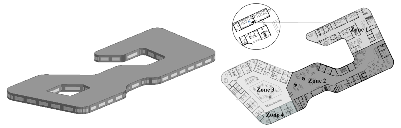
All illuminance, EML, and glare quantities reported in this study are evaluated at a single daylighting reference point, located in a patient room within Zone 1 at 1.2 m above the floor, corresponding to seated eye height, and shown in Figure 1. This zone is modelled as a 24 hour operation, so every simulated hour is treated as an occupied hour and the cooling and circadian aggregations are performed over all simulated hours.
2.2. City selection rationale
Jeddah, Athens, and Seattle were selected to span a deliberate gradient of cooling dominance rather than to represent any particular region comprehensively. Jeddah represents a cooling dominated climate in which the energy circadian trade-off that motivates this study was first identified and is expected to be strongest. Seattle represents the opposite end of the gradient, a heating leaning climate with minimal cooling demand, where the same trade-off mechanism would be expected to weaken or largely disappear if it is driven by cooling load rather than being an artifact of the optimization formulation itself. Athens was selected as an intermediate case with a mixed cooling and heating load profile, allowing the study to test whether the control strategy's behavior changes gradually for the gradient or shifts between two regimes. This three-point design was chosen specifically to test the climate transferability of the control strategy and the trade-off it manages, which is this study's central research question, rather than to provide exhaustive geographic coverage.
2.3. Simulation workflow setup
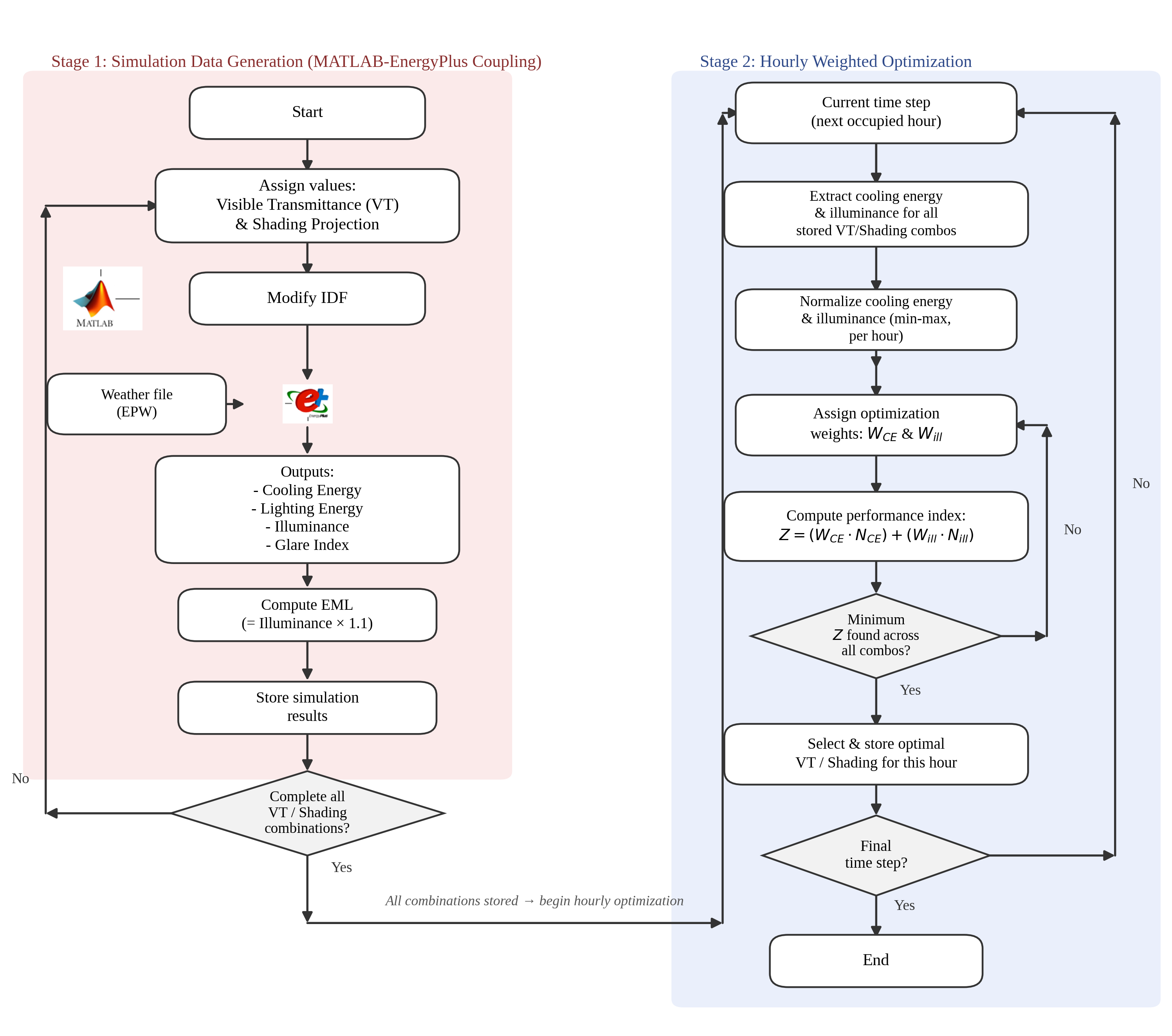
The simulation workflow couples EnergyPlus with MATLAB to perform hourly parametric and optimization analyses. The DesignBuilder model was developed using representative construction systems, fenestration (glazing type and orientation), and internal loads (occupancy, lighting, equipment) and HVAC, exported as an EnergyPlus Input Data File (IDF) for use in the MATLAB simulation environment. EnergyPlus performs the hourly simulations, daylight illuminance, cooling energy consumption, lighting energy use, and glare index throughout the building's zones, while MATLAB systematically modifies the key input parameters (visible transmittance and shading dimensions) and automates the workflow between EnergyPlus and the optimal control algorithm, extracting hourly outputs and processing them through the weighted multi-objective optimization algorithm described in Section 2.4.
For this three-climate comparison, the building model, zoning, internal loads, and HVAC configuration are identical for all three runs. The only substituted input is the EnergyPlus weather (EPW) file, sourced for all three cities from the EnergyPlus weather data repository [49]: Jeddah, Saudi Arabia (hot arid, cooling dominated); Athens, Greece (Mediterranean, mixed cooling and heating load); and Seattle, USA (marine west coast, heating leaning, low cooling load).
No independent validation against measured field data was performed for this study, consistent with its comparative, relative-trade-off scope for three climates rather than an absolute-performance claim for any single building. Model verification instead relies on EnergyPlus's own extensive validated test suite, including compliance with ASHRAE Standard 140 (Building Thermal Envelope and Fabric Load Tests), and on sanity-checking the resulting annual cooling energy intensities against the typical reported range for hospital buildings in each climate zone. A dedicated calibration against measured utility or monitored data for this specific hospital design was not within this study's scope and is identified as a direction for future work.
2.4. Parametric and optimization setup
Two design variables are controlled hourly: visible transmittance (VT), ranging between 0.1 and 0.8 in 0.1 increments, giving eight levels, and shading projection depth, ranging between 0.2 and 1.0 m in 0.2 m increments (0.2, 0.4, 0.6, 0.8, 1.0), giving five levels. The two variables together define a parametric grid of 40 combinations, which is the grid referred to throughout this paper, and the scan is discretized rather than continuous. For each combination, MATLAB assigns a VT and shading pair, updates the IDF, and EnergyPlus runs the hourly simulation using the climate specific EPW file, generating hourly cooling energy consumption, lighting energy demand, illuminance, and glare index. MATLAB then computes Equivalent Melanopic Lux (EML) from the illuminance data as shown in Eq. (1):
here, Ev is the illuminance at the daylighting reference point described in Section 2.1, and 1.1 is the melanopic ratio given for daylight at 6500 K in Table L1 of the WELL Building Standard v2 [2], which defines equivalent melanopic lux as the product of the photopic illuminance and that ratio. Eq. (1) is therefore a fixed coefficient approximation, and the quantity reported throughout this paper is a WELL v2 melanopic ratio estimate of EML rather than a spectrally resolved melanopic quantity computed per CIE S 026. It is evaluated against the WELL threshold of 200 EML for daytime spaces [2], which is defined on the same basis, and the limits of the approximation are stated in Section 4.3. The weighted multi-objective optimization balances cooling energy reduction against daylight availability via a performance index, as presented in Eq. (2):
where WCE and Will are weight coefficients for cooling energy and illuminance respectively, and NCE and Nill are the corresponding min-max normalized terms, computed per hour for the parametric grid as shown in Eq. (3) and Eq. (4):
so that NCE and Nill both equal 0 for the best achievable value at that hour and 1 for the worst. Where the range of a term for the 40 combinations in a given hour is zero, the denominator vanishes and the corresponding normalized term is set to zero for all combinations rather than evaluated, so that no division by zero occurs and a term that cannot discriminate between combinations contributes nothing to the objective in that hour. Where the objective is flat for all 40 combinations, the control state of the preceding hour is retained. This condition is not rare and its frequency differs sharply between the climates, as reported in Section 3.1. The weighting scheme is defined once here and referred to throughout: WCE takes 21 discrete values from 0.00 to 1.00 in increments of 0.05, with Will = 1 − WCE, so that the two weights always sum to one.
Glare is evaluated using the Daylighting Reference Point Glare Index reported by EnergyPlus, which is the Hopkinson daylight glare index (DGI) [50]. It is computed as shown in Eq. (5), following the EnergyPlus Engineering Reference [51]:
where Lw is the average luminance of the window as seen from the reference point, Ω is the solid angle subtended by the window modified by the Guth position index, ω is the solid angle subtended by the window with respect to the reference point, and Lb is the background luminance. The index is dimensionless. On the standard DGI scale, a value of 16 corresponds to just perceptible glare, 20 to just acceptable, 22 to the border between comfortable and uncomfortable, 24 to just uncomfortable, and 28 to just intolerable.
The optimization runs at hourly resolution for the full year for each of the three climates, with the control algorithm selecting the VT and shading combination that minimizes Z at each hourly time step. The selected state is assumed to be reached instantaneously and held for the hour. Motorised external shading typically repositions within seconds to a few minutes and electrochromic glazing typically switches within 5 to 20 minutes, both short relative to the hourly time step, but the model contains no actuation delay, no switching hysteresis, and no limit on the number of switching cycles per day. Figure 2 summarizes the complete workflow, from parametric simulation data generation through the hourly optimization search that produces the results reported in Section 3.
2.5. Data analysis methods
Outputs are compared for five dimensions for each climate: (1) the trade-off front between cooling energy and circadian performance for the full WCE weighting range; (2) the position of the dynamic control result within the static design space formed by the 40 fixed combinations; (3) seasonal hourly control profiles of VT and shading projection for representative winter, summer, and transition weeks; (4) annual hour of day by day of year control deployment patterns at a stated weighting; and (5) the glare weighted variant of the objective, evaluated against the WELL 200 EML threshold [2] and the IES recommended illuminance range for healthcare interiors of approximately 107.6 to 322.9 lux [52]. The core analytical contribution of this study is a cross-climate comparison layer applied to all five dimensions: the same performance metrics are computed identically for Jeddah, Athens, and Seattle and compared directly against one another to test whether the energy circadian trade-off's magnitude and shape, and the optimal control policy's seasonal behavior, are climate invariant or climate specific.
The representative weeks are 1 to 7 February for winter, 20 to 27 August for summer, and 12 to 18 October for the transition period. The transition week was selected quantitatively rather than assumed. For the unshaded reference configuration in Jeddah, the mean hourly cooling load over the week, expressed as a ratio of the annual mean hourly cooling load, is 0.21 for the winter week and 1.87 for the summer week, while the 12 to 18 October week gives 1.11 and therefore sits between the two. A mid April week was also tested and rejected because it produces zero cooling load in both Athens and Seattle, which makes it uninformative for a comparison whose subject is the cooling energy trade-off.
Two reporting conventions are applied throughout the Results. Annual energy quantities are reported as energy use intensity in kWh/m²/yr, while hourly distributions are reported in kWh/h, and every axis label, table header, and caption follows this distinction. Circadian compliance is reported over daylit hours, meaning hours in which the illuminance is non-zero for at least one of the 40 combinations, since 45.7% of the simulated hours are dark and can never meet a daylight based threshold. Aggregating over all hours would therefore cap the achievable compliance at the daylit fraction of the year, approximately 54%, and compress the differences between the climates. Mean EML is reported on both bases where the distinction matters.
3. Results
All results presented in this section were computed directly from the full 40 combination hourly parametric dataset (5 shading depths by 8 visible transmittance levels by 8,395 simulated hours per year) for each of the three climates. Cooling energy intensity is normalized by floor area (approximately 8,000 m²).
3.1. Trade-off Front Between Cooling Energy and Circadian Performance
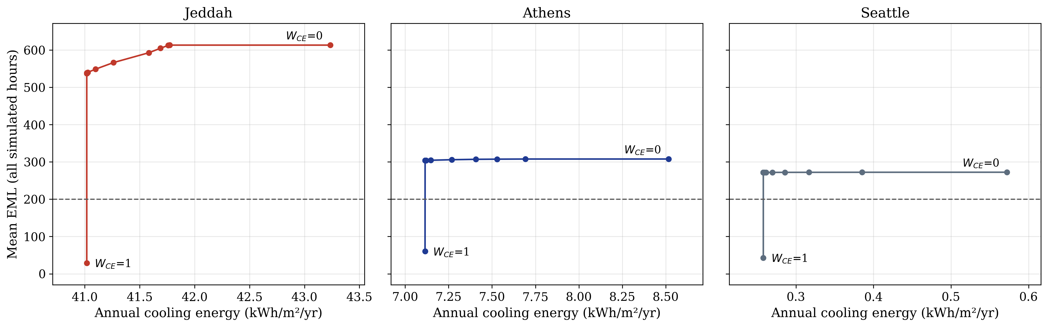
Table 1 summarizes the trade-off front endpoints for Jeddah, Athens, and Seattle. Figure 3 shows annual cooling energy intensity plotted against mean EML, one panel per climate, with the cooling energy weight WCE varied for the 21 weight points defined in Section 2.4. All three climates produce a strongly non-linear knee front: the optimizer holds circadian performance near its best achievable value while capturing nearly all available cooling energy savings for almost the entire weight range, with performance collapsing only at the single extreme where illuminance is given zero weight (WCE = 1.0). The horizontal scales differ between panels by roughly a factor of 75 between Jeddah and Seattle, so the shapes of the knees should not be compared directly by eye and are described quantitatively below.
| City | Cooling at WCE=0 (kWh/m2/yr) | Cooling at WCE=1 (kWh/m2/yr) | Max cooling reduction | Mean EML at WCE=0 | Mean EML at WCE=1 | % daylit hrs ≥ 200 EML at WCE=0 |
|---|---|---|---|---|---|---|
| Jeddah | 43.236 | 41.018 | 5.1% | 613.2 | 28.8 | 90.7% |
| Athens | 8.517 | 7.114 | 16.5% | 307.8 | 60.3 | 81.0% |
| Seattle | 0.572 | 0.258 | 54.9% | 272.4 | 42.7 | 74.8% |
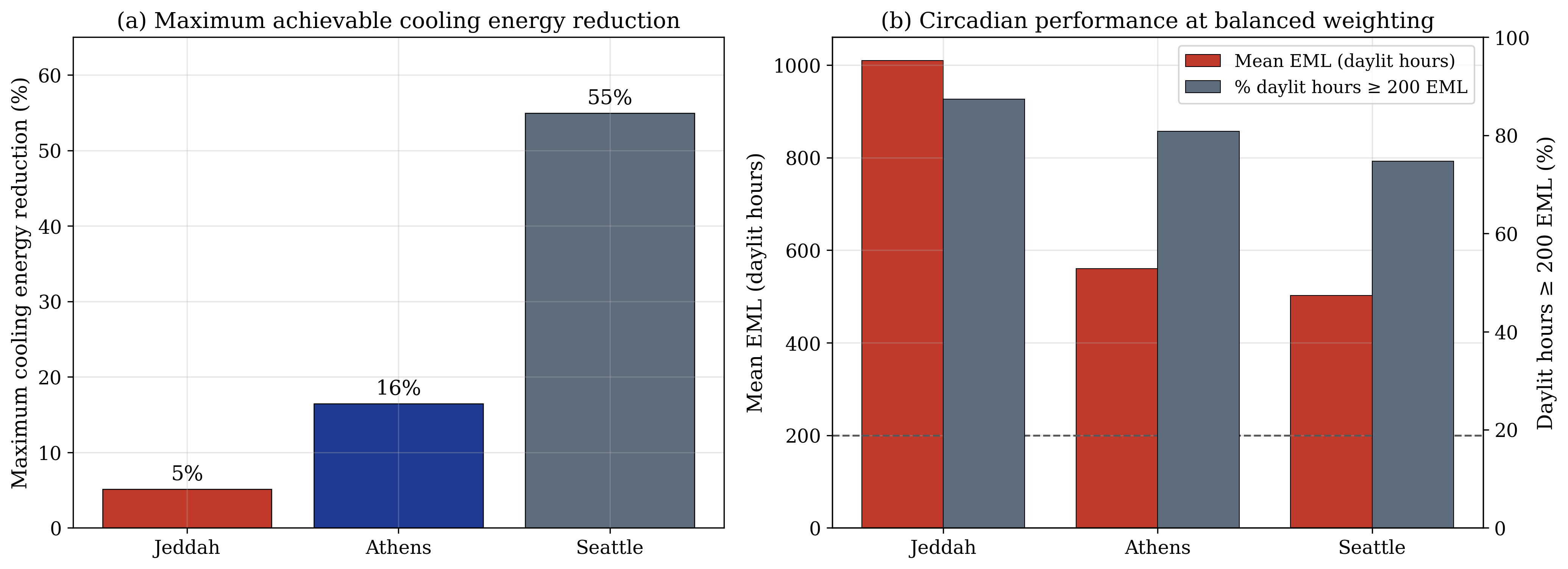
The achievable cooling energy reduction before the collapse scales inversely with a climate's cooling dominance: Jeddah gives up only 5% of its cooling energy before reaching the circadian limit, while Seattle, whose cooling load is minor, can cut it by 55% in relative terms, although the absolute saving is only 0.31 kWh/m²/yr and cooling is therefore not a design driver in that climate. This is confirmed directly by the frequency with which the envelope control has any influence on cooling at all. The cooling energy is identical for all 40 combinations, and the cooling term is therefore degenerate in the sense defined in Section 2.4, in 39.3% of the simulated hours in Jeddah, 78.4% in Athens, and 96.9% in Seattle. The illuminance term is degenerate in 45.7%, 45.7%, and 45.9% of hours respectively, and in every one of those hours the illuminance is zero for all combinations, so the condition corresponds exactly to the dark hours of the year.
Only Jeddah's front shows real interior curvature. Over the interior of the weighting range, from WCE of 0.30 to 0.55, mean EML in Jeddah declines steadily from 612.5 to 540.2 while annual cooling energy falls from 41.759 to 41.027 kWh/m²/yr, so intermediate weightings deliver intermediate outcomes. Athens and Seattle show almost no interior movement over the same interval: mean EML in Athens moves only from 304.1 to 304.0 and cooling energy from 7.121 to 7.117 kWh/m²/yr, and in Seattle neither quantity changes at the reported precision.
Athens and Seattle therefore show a small initial step within the first 0.25 of weight, a long flat stretch, and then the same sharp final step collapse, confirming that the interior of the weighting range carries usable resolution only in the cooling dominated climate. Section 4.1 presents the full interpretation.
3.2. Full design space
Figure 4 plots, for each city, the mean annual cooling energy and mean EML achieved by all 40 individual VT and shading combinations, each held fixed for the whole year with no hourly actuation, coloured by shading depth. This complements Figure 3 by showing the entire achievable static design space rather than only the optimized trajectory for it, and makes clear that shading depth, not visible transmittance, is the dominant driver of both cooling energy and EML in all three climates. The dynamic control result at balanced weighting is overlaid on each panel.
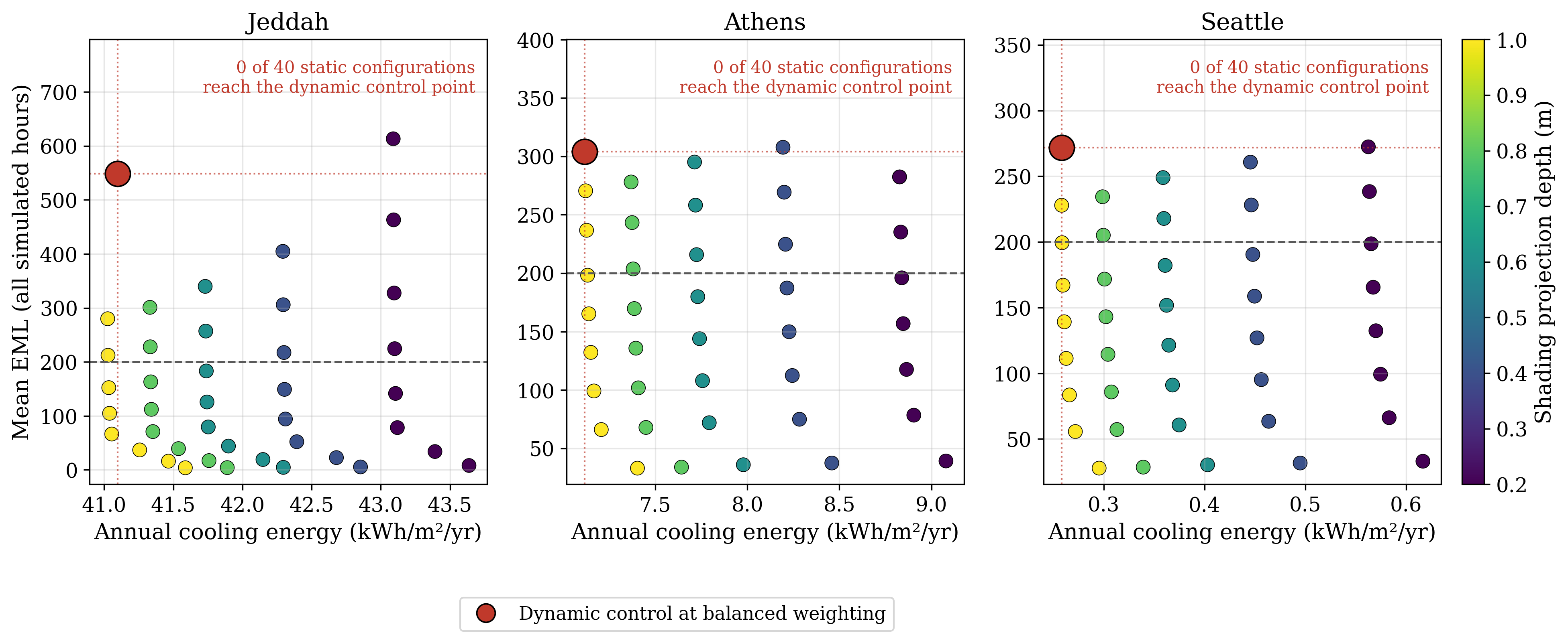
The overlay provides the absolute reference that a comparison expressed only relative to the weighting scheme cannot give. In all three climates, no static configuration in the design space achieves the combination of cooling energy and mean EML delivered by the dynamic control: of the 40 fixed combinations, zero match or better it on both axes simultaneously. Figure 5 and Table 2 report the comparison against a static reference of 0.2 m projection and VT 0.8, representing clear glazing without meaningful external shading and held fixed for the whole year. Against that reference the dynamic strategy reduces annual cooling energy by 4.6% in Jeddah, 19.4% in Athens, and 54.2% in Seattle, while mean EML changes by -10.5%, +7.6%, and -0.2% respectively, so that almost the whole cooling saving is obtained at essentially unchanged circadian performance. The saving scales with cooling dominance in the same direction as the trade-off front itself.
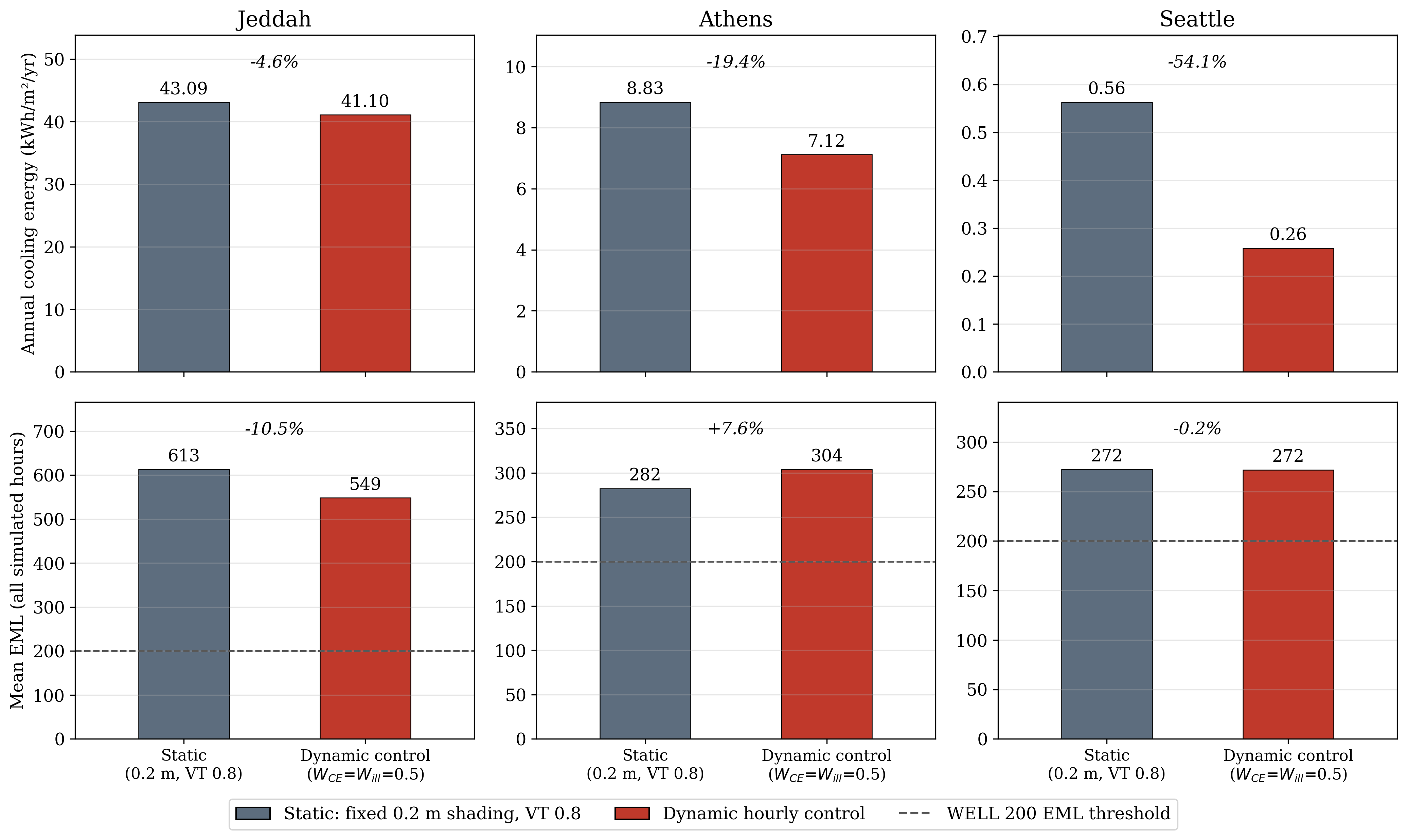
| Case | Jeddah cooling | Jeddah EML | Athens cooling | Athens EML | Seattle cooling | Seattle EML |
|---|---|---|---|---|---|---|
|
Static (0.2 m, VT 0.8) |
43.090 | 613.2 | 8.827 | 282.5 | 0.563 | 272.4 |
| Dynamic control (WCE = Will = 0.5) | 41.097 | 548.6 | 7.117 | 304.0 | 0.258 | 271.8 |
3.3. Seasonal hourly control profiles
Figure 6 and Figure 7 show visible transmittance and shading projection for representative winter (Feb 1 to 7), summer (Aug 20 to 27), and transition (Oct 12 to 18) weeks for all three climates, under cooling prioritized (WCE = 0.8) and daylight prioritized (WCE = 0.2) weighting respectively. Under daylight prioritized weighting, all three cities keep VT at or near its maximum through daylit hours. The seasonal contrast is where the climates diverge: Jeddah and Athens both show a clear winter and summer asymmetry, while Seattle's seasonal swing is visibly smaller and shallower for all three representative weeks. Under cooling prioritized weighting, shading becomes the dominant control variable in all three cities, but the frequency and depth of shading deployment scales down from Jeddah through Athens to Seattle.
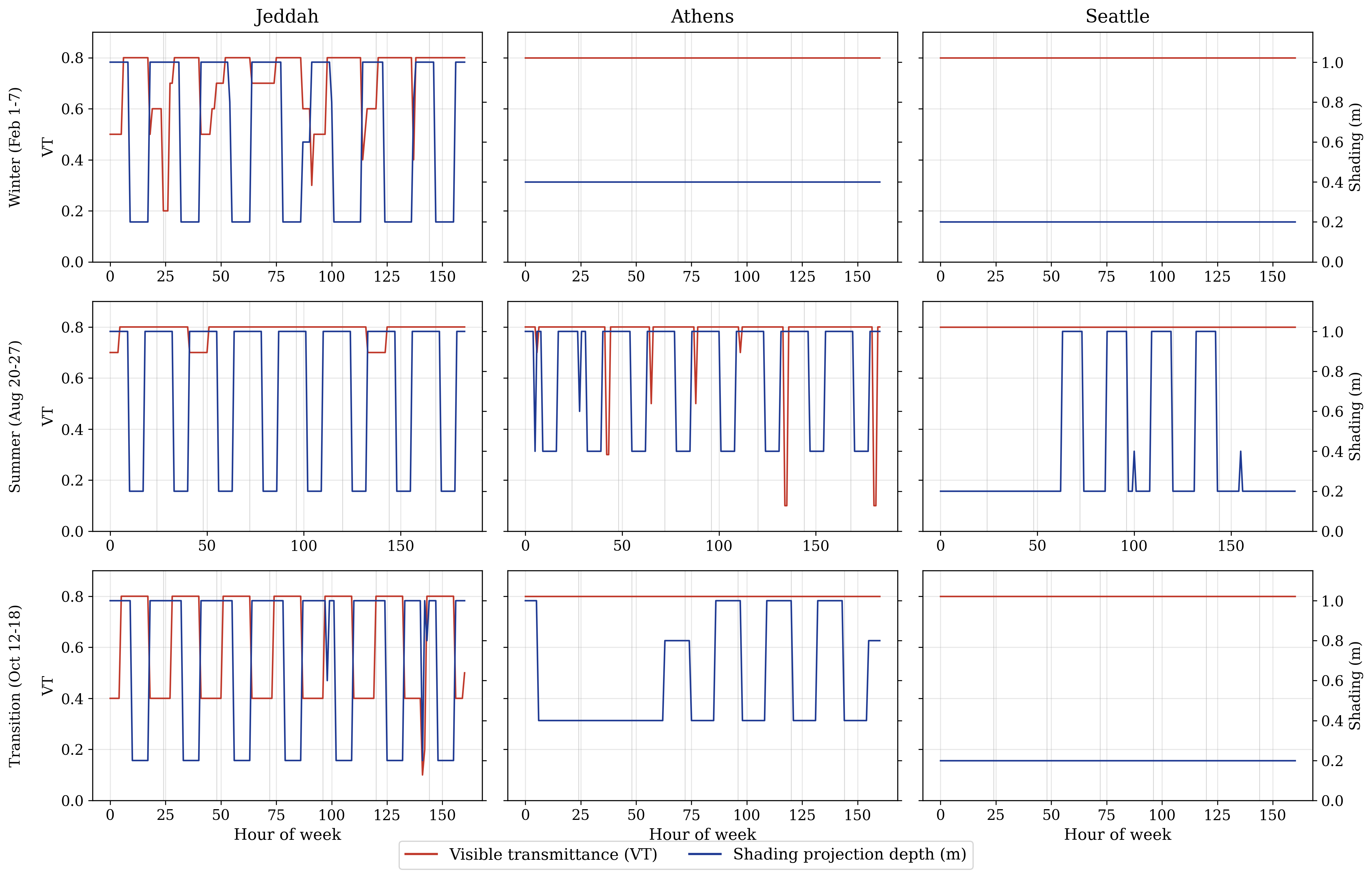
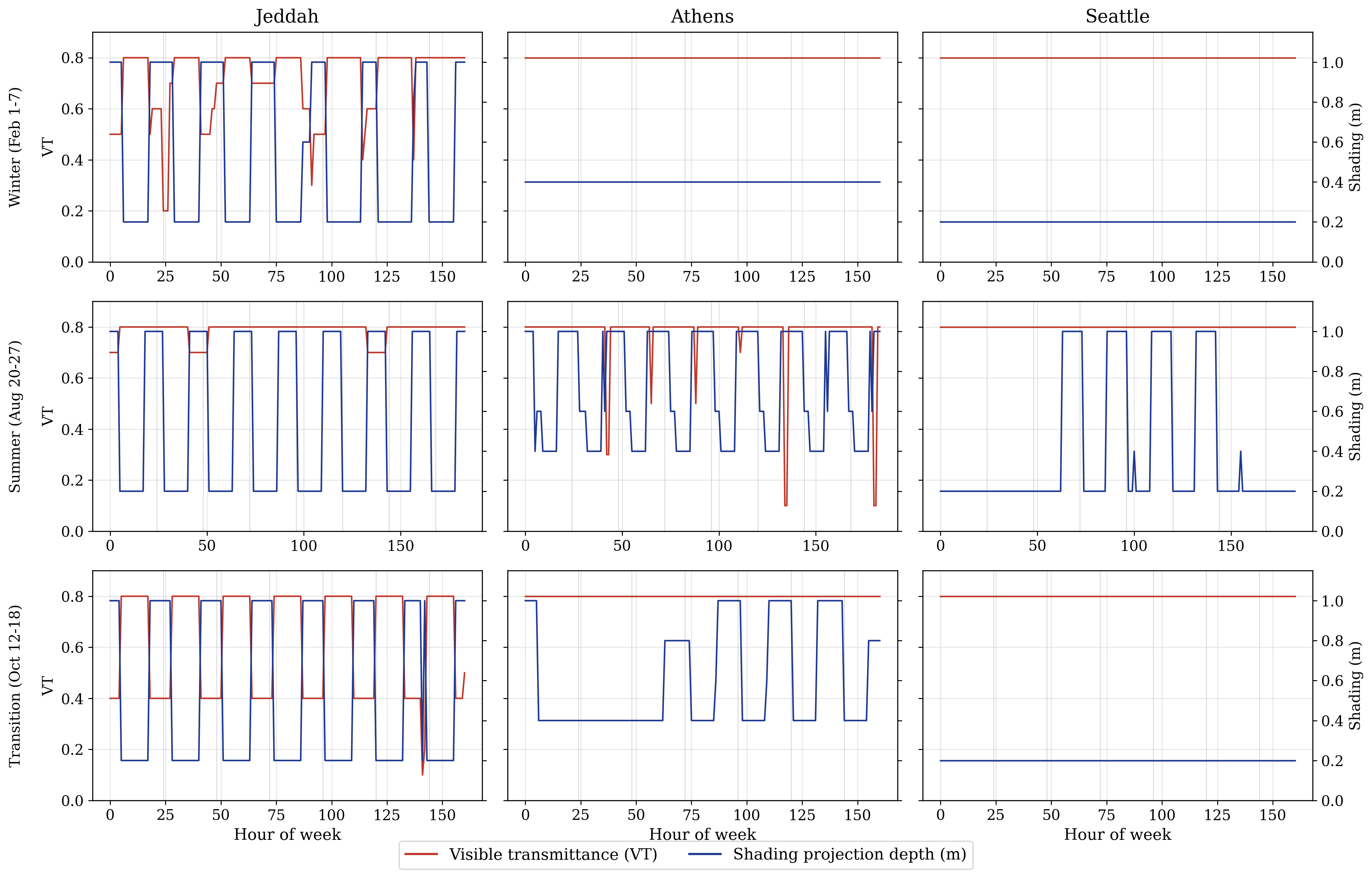
The two weighting scenarios produce control profiles that are close to identical over these weeks. Comparing the two hourly paths hour by hour, the selected shading depth is the same in 81% of the plotted hours in Jeddah, 94% in Athens, and 100% in Seattle, and the selected visible transmittance is the same in 100%, 99.8%, and 100% respectively. The weighting therefore changes the control policy only in a minority of hours, which is the same insensitivity that produces the long flat stretch of the trade-off front in Section 3.1.
3.4. Annual dynamic operation of the control system
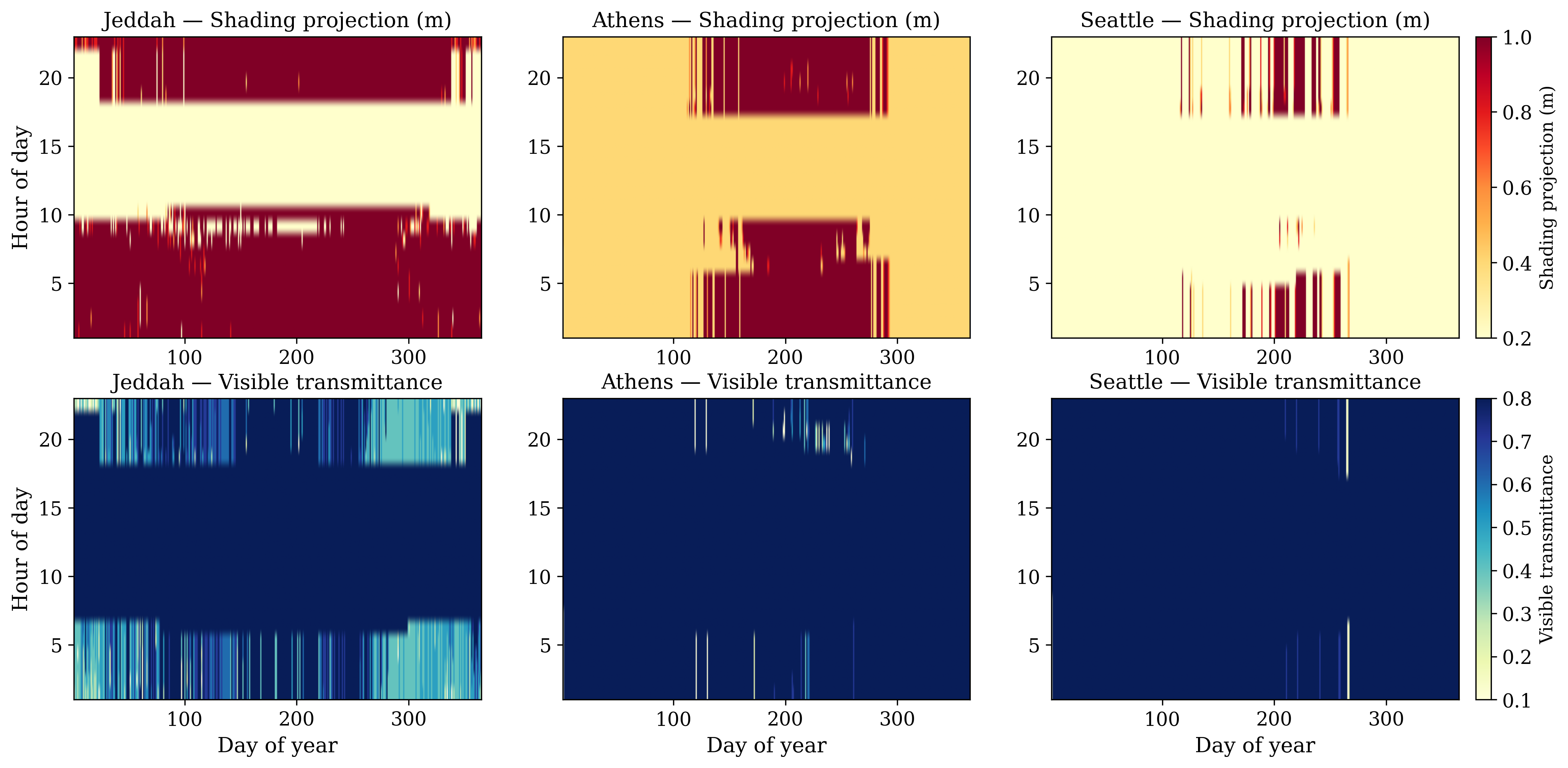
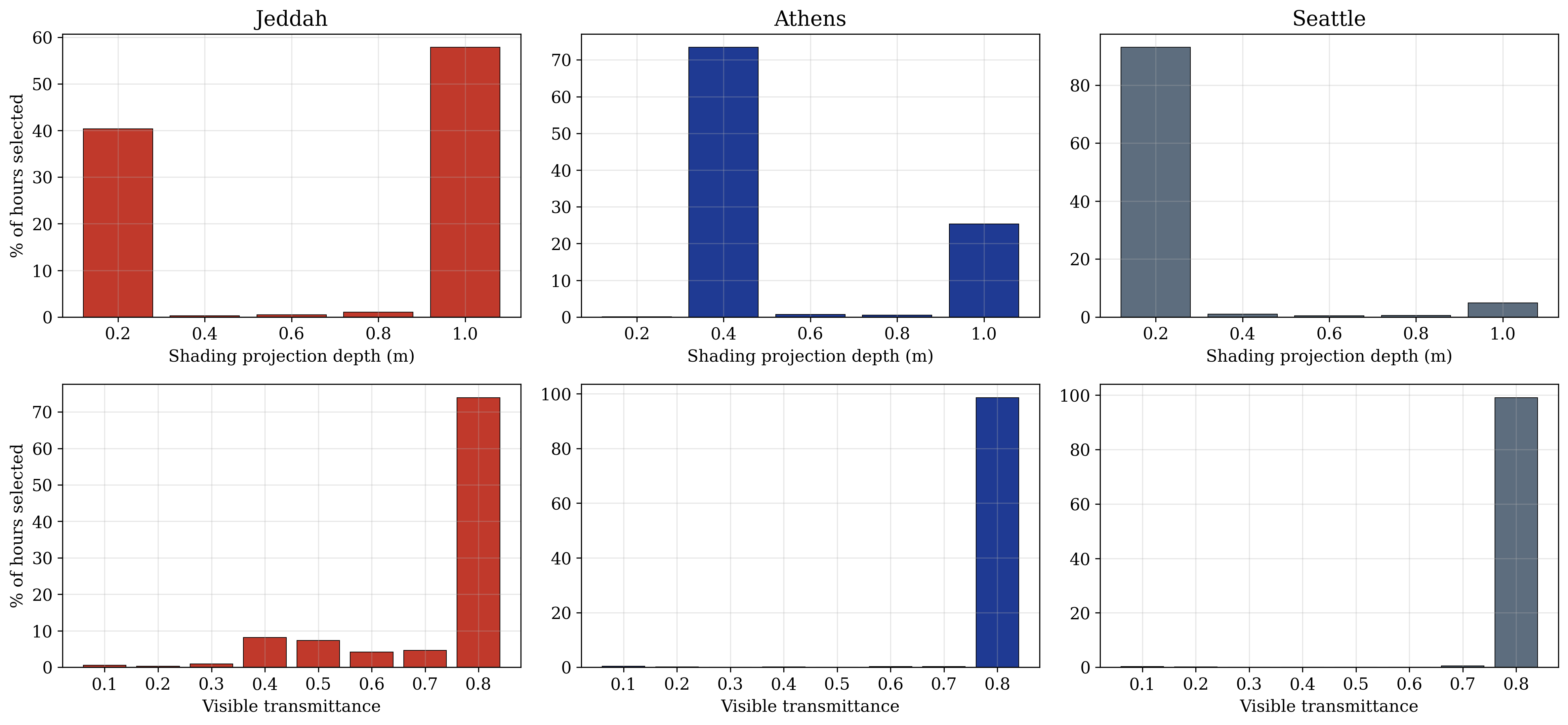
Figure 8 shows annual heatmaps of optimal shading depth and visible transmittance by hour of day and day of year, computed at a balanced weighting (WCE = Will = 0.5) for all three cities. This is the clearest cross-climate result in the dataset, forming a three-step gradient in the overall intensity of shading use: the annual mean shading projection is 0.67 m in Jeddah, 0.56 m in Athens, and 0.25 m in Seattle. Jeddah deploys shading at or near maximum depth through the great majority of hours in which daylight is unavailable, holding 1.0 m in 89.7% of those hours year-round, and withdraws it during the daylit hours, holding the minimum 0.2 m in 67.7% of them, so that the daylight available to the circadian objective is preserved when it exists and cooling is minimized when it does not. Athens shows an intermediate pattern, with a moderate 0.4 m shading baseline held through most daylit hours year-round, 73.4% of all simulated hours, and escalation to maximum depth in the early morning and evening shoulder hours during a wide summer band. Seattle deploys shading only in a narrow summer evening window, remaining at the minimum depth in 93% of all simulated hours.
3.5. Monthly distribution of cooling energy and EML
Figure 9 shows monthly box plots of hourly cooling energy and EML at balanced weighting for the three climates.
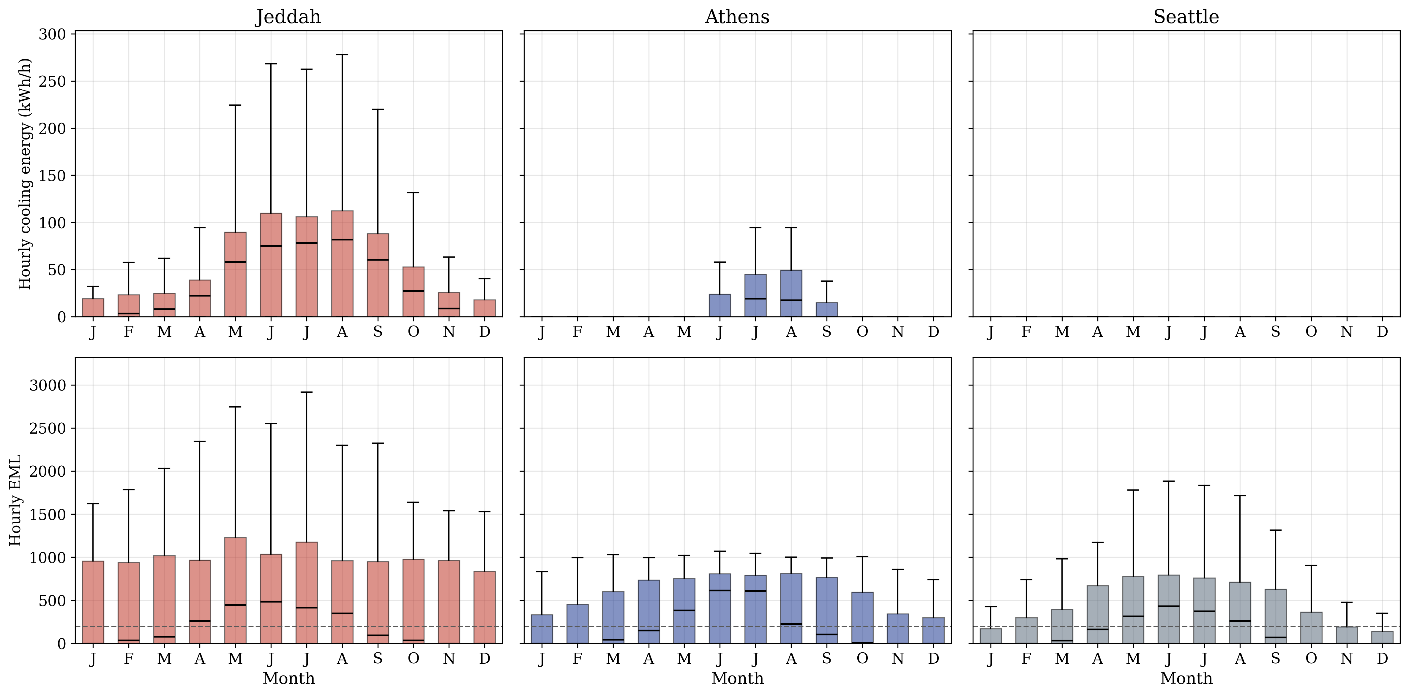
These complement the annual heatmaps in Section 3.4 by quantifying the spread, not just the mean, of each metric within each month. Jeddah's cooling energy distribution is comparatively narrow and high year-round, consistent with a cooling load present in every month. Athens shows a wider seasonal swing in the median, with summer months showing both a higher median and greater within month variability. In Seattle the median and the interquartile range of hourly cooling energy are zero in every month, so the boxes collapse onto the zero line, and cooling occurs only in sparse summer hours that fall outside the plotted range. EML distributions are comparatively stable for months within each city relative to their cooling energy counterparts, consistent with the trade-off front shape in Figure 3, the optimizer protects circadian performance for most of the weighting range regardless of season.
3.6. Control-variable discretization frequency
Figure 10 shows how often each of the five discrete shading depths and eight discrete VT levels is selected as optimal at balanced weighting, for all three climates. This diagnostic view, not typically reported in similar studies, shows whether the discretized parametric grid used in this study (Section 2.4) is fine enough to avoid concentrating the optimizer's choices onto only one or two extreme levels. In all three cities, shading depth selection is bimodal, concentrated at the minimum (0.2 m) and maximum (1.0 m) levels with comparatively minimal use of intermediate depths, while VT selection is more distributed for the available range, particularly in Jeddah.
3.7. EML Duration Curve and Circadian Compliance Summary
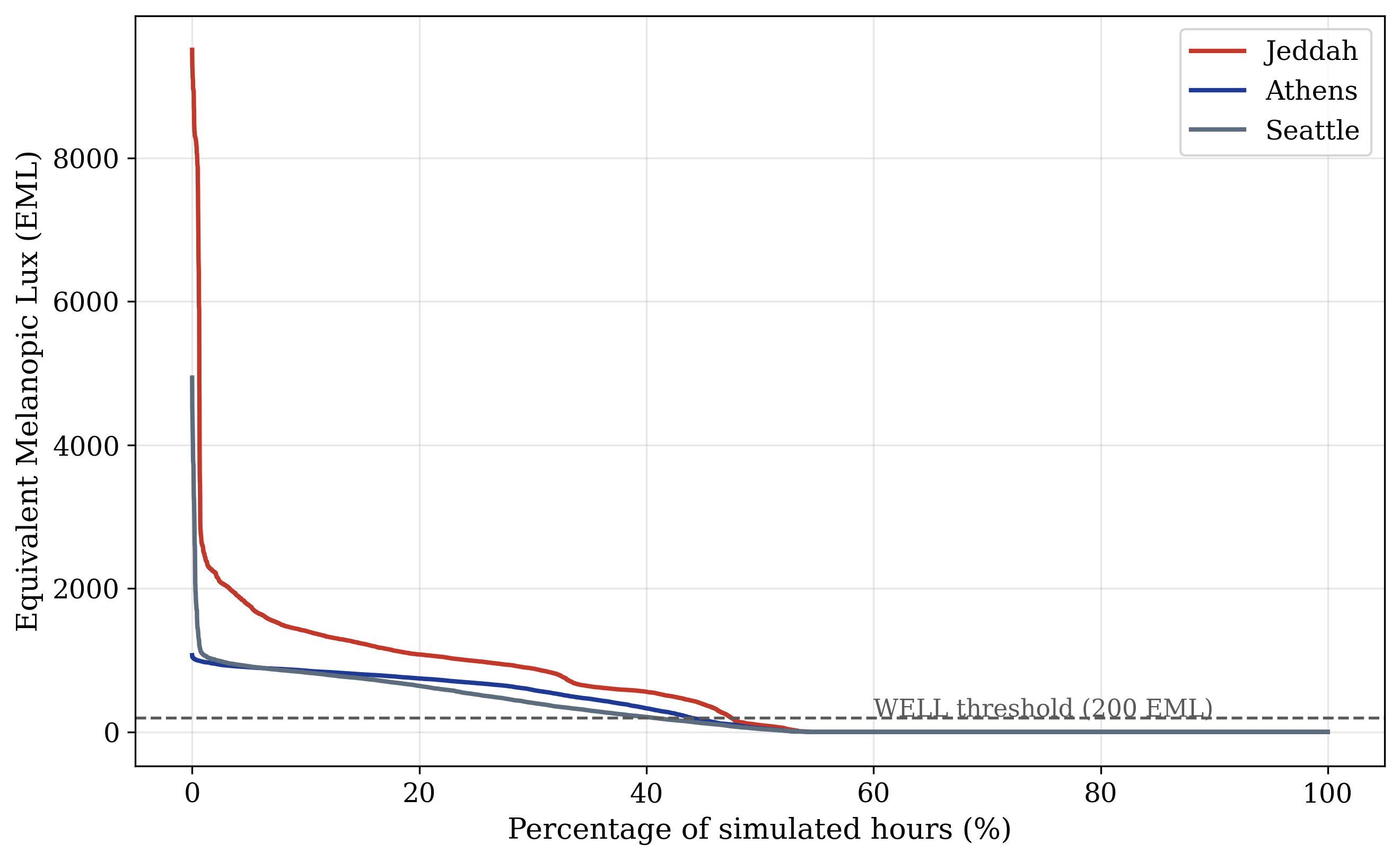
Figure 11 shows the EML duration curve, hours sorted by descending EML and expressed as a percentage of the simulated year, at balanced weighting for all three climates on shared axes. Figure 12 summarizes the maximum achievable cooling energy reduction by climate together with mean EML and the percentage of daylit hours meeting the WELL 200 EML threshold. Table 3 presents the corresponding circadian compliance values at balanced weighting for the three climates. Reported over daylit hours, the basis defined in Section 2.5, the three climates separate clearly: 87.4% of daylit hours meet the WELL 200 EML threshold in Jeddah, 80.8% in Athens, and 74.7% in Seattle, with mean daylit hour EML of 1,010, 560, and 502 respectively. The ordering follows daylight availability rather than cooling energy demand, and the spread between the three climates is far narrower than the roughly 75 fold difference in absolute cooling energy demand between Jeddah and Seattle documented in Table 1.
| City | Mean EML (all hours) | Mean EML (daylit hours) |
% daylit hours ≥ 200 EML |
|---|---|---|---|
| Jeddah | 548.6 | 1009.6 | 87.4% |
| Athens | 304.0 | 560.1 | 80.8% |
| Seattle | 271.8 | 502.4 | 74.7% |
Circadian performance under this control strategy is therefore substantially decoupled from a climate's cooling energy magnitude for most of the practical weighting range.
3.8. Glare-weighted optimization variant
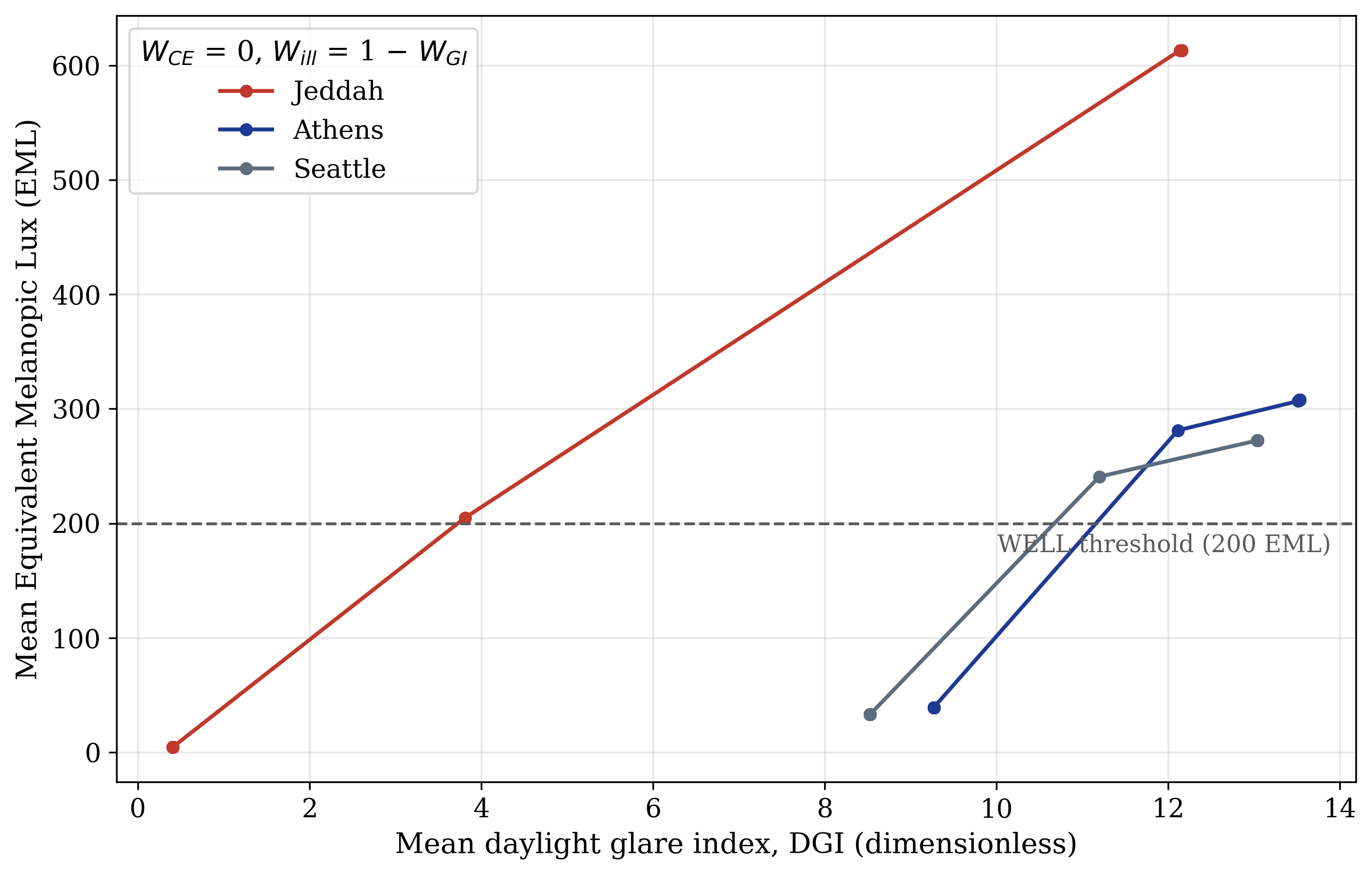
Figure 13 shows the mean daylight glare index achieved plotted against mean EML for all three climates on shared axes, varying WGI for its full range with WCE = 0 and Will = 1 − WGI as defined in Section 2.4. Table 4 summarizes mean EML over daylit hours at selected glare weights for each climate. All three climates show the same qualitative behavior: once glare weighting crosses roughly WGI of 0.5 to 0.6, the optimizer sharply cuts VT and illuminance to control glare, and mean EML falls below the WELL 200 EML threshold in all three climates. Both quantities are reported over daylit hours, since the dark hours return a glare index of zero and would otherwise dominate the annual mean.
| City | WGI=0.3 (pre-collapse) | WGI=0.5 (transition) | WGI=0.6 (post-collapse) |
|---|---|---|---|
| Jeddah | 1128.4 | 376.9 | 8.1 |
| Athens | 567.0 | 518.1 | 72.2 |
| Seattle | 503.5 | 445.1 | 61.2 |
Jeddah's collapse is the most extreme of the three, from 1,128 to 8 EML over daylit hours. This is the most climate independent finding in the whole comparison, since glare prioritized control defeats the circadian objective everywhere and not only in hot arid conditions. At the daylight prioritized end of the range, where the objective places no weight on glare at all, the mean daylit hour DGI reaches 22.4 in Jeddah, 24.9 in Athens, and 24.1 in Seattle, at or above the just uncomfortable level on the scale given in Section 2.4. Controlling glare is therefore a requirement of any practical deployment of this strategy rather than an optional refinement.
4. Discussion
4.1. Discussion of results
The three-climate Pareto front comparison presented in Section 3.1 answers the central question of this study, characterizing not just whether the trade-off exists but what shape it takes in each climate. All three climates share the same qualitative shape, a sharp knee in which the optimizer keeps circadian performance near its maximum while capturing nearly all the achievable cooling savings over almost the entire weighting range, dropping off only at the single extreme where illuminance is given zero weight. The climates differ sharply in two ways that matter for this study's contribution. First, the cooling saving available before the drop-off scales inversely with cooling dominance: Jeddah, cooling dominated, gives up only 5% of its cooling energy before circadian performance falls; Athens, mixed load, gives up 17%; and Seattle, heating leaning, gives up 55% in relative terms, since its cooling demand starts out small at around 0.57 kWh/m²/yr. Second, only Jeddah's front shows real interior curvature, a gradual decline in EML over the middle of the weighting range (WCE of about 0.30 to 0.55) before the final drop, while Athens and Seattle move almost directly from protecting daylight to giving it up entirely, with very small intermediate ground available for adjustment. This supports the study's central idea: the energy circadian trade-off is not simply larger in cooling dominated climates, its shape is different too, a continuously tunable trade-off in Jeddah compared with a near binary choice in Athens and Seattle.
The degenerate hour fractions reported in Section 3.1 give the mechanism behind this difference directly. In Seattle the cooling energy is identical for all 40 combinations in 96.9% of simulated hours, and in Athens in 78.4%, against 39.3% in Jeddah. In those hours the cooling term contributes nothing to the objective whatever weight it carries, so the control state is determined by the illuminance term alone and the weighting has no effect until it becomes extreme. A near binary front is therefore the expected consequence of a climate in which the envelope has almost no influence on cooling for most of the year, and the interior curvature seen in Jeddah requires a cooling load that the envelope can actually act on for a large share of hours.
The annual heatmap finding in Section 3.4 is consistent with the same mechanism. Shading use forms a clear three-step gradient in annual mean projection depth, 0.67 m in Jeddah, 0.56 m in Athens, and 0.25 m in Seattle, and the within-day pattern is common to all three: the controller withdraws shading while daylight is available and deploys it when daylight is absent and only the cooling term remains active. Jeddah's cooling load is present in every month and every hour, so this pattern is expressed strongly and year-round. Seattle's cooling load is small enough that there is rarely anything for the shading to act on, so the policy stays close to its minimum state throughout. The practical reading is that the control logic itself is climate invariant while the intensity with which it operates is not.
The glare weighted variant remains the most climate independent result in the comparison. Once glare priority crosses roughly WGI of 0.5 to 0.6, every climate collapses to EML values far below the WELL threshold, Jeddah most severely (1,128 to 8), followed by Athens (567 to 72) and Seattle (504 to 61). Unlike the cooling energy trade-off, the glare against circadian trade-off does not weaken in a low cooling load climate, since glare depends on solar geometry and sky brightness rather than on cooling demand. This is the most transferable finding in this study, and it carries a direct design implication, since the glare weight is the one parameter of this control strategy that cannot be tuned aggressively in any market without defeating the circadian objective it is meant to serve.
4.2. Comparison with literature
The finding that optimal envelope and shading behavior differs sharply by climate is consistent with the broader multi-climate optimization literature, in which climate specific optimal configurations for energy and daylight objectives are reported consistently [8,9,11], though none of that work includes a circadian or melanopic term, which is precisely the gap this study fills. The systematic review presented in [35] found that meeting circadian lighting recommendations can substantially increase electric lighting energy use; this study's results extend that logic to cooling energy specifically and show, for the first time in a multi-climate hourly optimization framework, that the size of the penalty is climate dependent rather than fixed. The study reported in [34] is the closest existing methodological precedent, evaluating useful daylight illuminance, circadian stimulus, and energy performance in a multi-objective optimization of thermochromic glazing, but for a single location and a different envelope technology; this study's cross-climate, shading and visible transmittance framing is the natural extension that single location precedent was missing. The near total absence of shading activity in Seattle for most of the year is also a concrete illustration of the comparative, climate based evaluation that the review in [36] found largely absent from the circadian daylighting literature.
4.3. Limitation
This study has several limitations. First, Eq. (1) applies a fixed melanopic ratio of 1.1, which assumes a D65 daylight spectrum and therefore cannot represent the variation of daylight spectrum with sky condition, solar altitude, glazing spectral transmittance, or interior surface reflectance; a spectrally resolved calculation following CIE S 026 would require spectral sky data and a spectral daylight simulation engine for all three sites and is identified as the principal direction for future work. Second, EML is derived from the illuminance at the daylighting reference point rather than from a separately computed vertical illuminance at the eye, which is the plane on which the WELL threshold is defined. Third, the static reference reported in Section 3.2 is a fixed configuration of the same envelope, so it isolates the contribution of dynamic actuation; a baseline built on a different glazing construction, such as a single glazed reference, would require a separate set of simulations and remains future work. Fourth, the building model, internal loads, and HVAC configuration are held identical for all three climates by design, which isolates the climate effect but also means the results describe how one specific hospital design responds to different climates rather than how a climate optimized design would perform in each location, and they should not be read as a claim about optimal hospital design per climate. Fifth, the control model assumes instantaneous switching with no actuation delay, no hysteresis, and no limit on switching cycles, as stated in Section 2.4. Sixth, the Pareto fronts are sampled at 21 discrete weight points, so the sharpness of the final step collapse could in principle reflect the coarseness of the sampling rather than a true discontinuity, and a finer resolution near WCE approaching 1 would confirm whether the collapse is a cliff or a very steep continuous decline. Finally, only three climates were evaluated, so the climate dependence claim, that both the achievable cooling reduction potential and the front's interior curvature scale with cooling dominance, is directional rather than a relationship fitted for a continuous climate gradient.
5. Conclusion
This study applied a single hourly, EnergyPlus and MATLAB weighted multi-objective control framework, targeting cooling energy and circadian effective daylight (EML), identically for three climatically distinct hospital sites: Jeddah (hot arid, cooling dominated), Athens (Mediterranean, mixed load), and Seattle (marine, heating leaning). Across the full weighting range, all three climates produced a strongly non-linear knee trade-off front in which circadian performance stays near its maximum while nearly all achievable cooling savings are obtained, collapsing only at the single extreme where daylight is given zero weight. The achievable cooling energy reduction before that collapse scaled inversely with cooling dominance, 5% in Jeddah, 17% in Athens, and 55% in Seattle in relative terms, and only Jeddah's front showed interior curvature, meaning that a truly tunable trade-off exists only where cooling load is substantial, while Athens and Seattle behaved in a near binary manner. The fraction of hours in which the envelope has no influence on cooling at all, 39.3% in Jeddah against 96.9% in Seattle, accounts for this difference directly, and it also shows that cooling is not a design driver in the Seattle case, where the 55% reduction corresponds to an absolute saving of only 0.31 kWh/m²/yr. Measured against the static design space, no fixed configuration out of 40 reached the combination of cooling energy and EML delivered by the dynamic control in any of the three climates. The annual control deployment pattern mirrored the climate gradient in intensity, with annual mean shading projections of 0.67 m, 0.56 m, and 0.25 m, while the within-day logic was common to all three, withdrawing shading while daylight is available and deploying it when it is not. The glare weighted variant was the one climate independent result, with glare control prioritized above a weight of roughly 0.5 to 0.6 collapsing circadian performance below the WELL 200 EML threshold in all three climates, most severely in Jeddah.
To the best of the authors' knowledge, based on a systematic literature search, this is the first study to evaluate an hourly, EnergyPlus coupled optimization strategy that targets cooling energy and circadian effective daylight for more than one climate, and the first to characterize the shape, not just the magnitude, of that trade-off as a function of climate. Three extensions follow directly from this work. Evaluating a broader climate gradient would allow the cooling dominance relationship to be fitted rather than stated directionally, and would clarify where the transition from tunable to near binary trade-off behavior occurs. A spectrally resolved melanopic calculation would replace the fixed ratio approximation used here and would test whether the absolute circadian gradient between climates survives the change of metric. Finally, a baseline built on a conventional single or double glazed construction, matching the definitions used in this framework, would extend the absolute comparison beyond the fixed configurations of the present envelope.
Funding
This research received no external funding.
Declaration of competing interest
The authors declares no conflicts of interest.
References
- R. J. Lucas et al., Measuring and using light in the melanopsin age, Trends in Neurosciences, 37:1 (2014) 1-9.
- International WELL Building Institute (IWBI), WELL Building Standard, v2, IWBI: New York, NY, USA, 2020.
- International Commission on Illumination (CIE), CIE System for Metrology of Optical Radiation for ipRGC-Influenced Responses to Light, CIE S 026/E:2018, CIE: Vienna, Austria, 2018.
- T. M. Brown et al., Recommendations for daytime, evening, and nighttime indoor light exposure to best support physiology, sleep, and wakefulness in healthy adults, PLoS Biology, 20:3 (2022) e3001571.
- M. S. Rea and M. G. Figueiro, Light as a circadian stimulus for architectural lighting, Lighting Research & Technology, 50:4 (2018) 497-510.
- W. Truong, B. Zandi, V. Q. Trinh, and T. Q. Khanh, Circadian metric - Computation of circadian stimulus using illuminance, correlated colour temperature and colour rendering index, Building and Environment, 184 (2020) 107146.
- S. I. Yun, J. W. Jeong, and A. Choi, Photopic illuminance-based black-box model for regulation of human circadian rhythm via daylight control, Building and Environment, 203 (2021) 108069.
- J. Zhao and Y. Du, Multi-objective optimization design for windows and shading configuration considering energy consumption and thermal comfort: A case study for office building in different climatic regions of China, Solar Energy, 206 (2020) 997-1017.
- M. Talaei and H. Sangin, Multi-objective optimization of energy and daylight performance for school envelopes in desert, semi-arid, and mediterranean climates of Iran, Building and Environment, 255 (2024) 111424.
- H. Wu and T. Zhang, Multi-objective optimization of energy, visual, and thermal performance for building envelopes in China's hot summer and cold winter climate zone, Journal of Building Engineering, 59 (2022) 105034.
- P. K. Chaturvedi et al., Multi-objective optimization of glazing and shading configurations for visual, thermal, and energy performance of cooling dominant climatic regions of India, Clean Technologies and Environmental Policy, 27:9 (2025) 4909-4932.
- H. Zhang et al., Optimization of the dynamic external shading control for railway stations in China based on energy use intensity (EUI) of lighting and HVAC systems, Buildings, 14:12 (2024) 3886.
- H. Dong, S. Vanage, and K. Cetin, Sensitivity analysis of sensor placement in energy-efficient, grid-interactive ready small office buildings with dynamic shading and lighting control, Science and Technology for the Built Environment, 30:5 (2024) 433-451.
- A. A. Bahdad et al., Parametric optimization approach to evaluate dynamic shading within double-skin insulated glazed units for multi-criteria daylighting performance in tropics, Journal of Daylighting, 11 (2024) 349-371.
- W. Lu, Dynamic shading and glazing technologies: Improve energy, visual, and thermal performance, Energy and Built Environment, 5:2 (2022) 211-229.
- A. Bertini et al., Control algorithm for dynamic solar shadings: A simulation study for office buildings based on ISO 52016-3, Building and Environment, 262 (2024) 111818.
- R. Roshan Kharrat, G. M. Perfetto, R. Ingaramo, and G. Mutani, Optimizing building performance with dynamic photovoltaic shading systems: A comparative analysis of six adaptive designs, Smart Cities, 8:4 (2025) 127.
- S. Chen, Z. Chen, and Y. Chen, Dynamic optimization model for passive solar shading and its application in building energy efficiency across multiple latitudes, Buildings, 16:10 (2026) 1887.
- C. Magraoui et al., A smart roller shutters control for enhancing thermal comfort and sustainable energy efficiency in office buildings, Sustainability, 17:5 (2025) 2116.
- M. Brzezicki, Enhancing daylight comfort with climate-responsive kinetic shading: A simulation and experimental study of a horizontal fin system, Sustainability, 16:18 (2024) 8156.
- N. Heidari Matin and A. Eydgahi, A data-driven optimized daylight pattern for responsive facades design, Intelligent Buildings International, 14:3 (2022) 363-374.
- D. A. Chi, An approach to determine specific targets of daylighting metrics and solar gains for different climatic regions, Journal of Daylighting, 8:1 (2021) 1-19.
- S. Li, D. H. W. Li, W. Chen, S. Lou, and E. K. W. Tsang, Simple mathematical models to link climate-based daylight metrics with daylight factor metrics and daylighting design implications, Heliyon, 9 (2023) e15786.
- T. Dogan and Y. C. Park, Testing the residential daylight score: Comparing climate-based daylighting metrics for 2444 individual dwelling units in temperate climates, Lighting Research & Technology, 52:8 (2020) 991-1008.
- C. Qiu and H. Yang, Daylighting and overall energy performance of a novel semi-transparent photovoltaic vacuum glazing in different climate zones, Applied Energy, 276 (2020) 115414.
- M. Talaei and H. Sangin, Comprehensive assessment of energy, daylight and visual comfort of rooftop and shading building-integrated photovoltaics across desert, steppe, and Mediterranean climates, Advances in Building Energy Research, 20:1 (2025) 62-103.
- B. Gaber, C. Zhan, X. Han, M. Omar, and G. Li, Enhancing daylight and energy efficiency in hot climate regions with a perforated shading system using a hybrid approach considering different case studies, Buildings, 15:6 (2025) 988.
- Z. Wu, Y. Xu, and Z. Wang, Multi-objective optimization of energy, view, daylight and thermal comfort for building's fenestration and shading system in hot-humid climates, PLOS ONE, 20:6 (2025) e0325290.
- G. Garcia-Martin, M. A. Campano, P. Bustamante, and I. Acosta, New approaches in dynamic metrics for lighting control systems: A critical review, Applied Sciences, 15:15 (2025) 8243.
- F. Fallahi, F. Ahmadi, M. Khakzand, and Y. Shahbazi, Designing a kinetic facade to control glare: Inspiration of long-day plants pattern, Journal of Daylighting, 12:2 (2025) 265-277.
- J. Mardaljevic, R. Kelly Waskett, and B. Painter, Neutral daylight illumination with variable transmission glass: Theory and validation, Lighting Research & Technology, 48:3 (2016) 267-285.
- D. Caicedo and A. Pandharipande, Daylight and occupancy adaptive lighting control system: An iterative optimization approach, Lighting Research & Technology, 48:6 (2016) 661-675.
- A. Pandharipande and G. R. Newsham, Lighting controls: Evolution and revolution, Lighting Research & Technology, 50:1 (2018) 115-128.
- L. Fan, L. Xie, and Q. Zhong, Multi-objective optimization of thermochromic glazing: Evaluating useful daylight illuminance, circadian stimulus, and energy performance with implications for sleep quality improvement, Energy and Buildings, 333 (2025) 115460.
- M. Taghizadeh, N. Gentile, P. Mattsson, and M. C. Dubois, Energy impact of integrative lighting: A systematic literature review, Energy and Buildings, 344 (2025) 115920.
- N. Ghaeili Ardabili, J. Wang, and N. Wang, A systematic literature review: Building window's influence on indoor circadian health, Renewable and Sustainable Energy Reviews, 188 (2023) 113796.
- R. Alelwani, Multi-objective optimization of window-to-wall ratio and shading devices for energy-efficient daylighting in Saudi residential villas, Discover Sustainability, 7:1 (2026) 539.
- C. S. Pechacek, M. Andersen, and S. W. Lockley, Preliminary method for prospective analysis of the circadian efficacy of (day)light with applications to healthcare architecture, LEUKOS, 5:1 (2008) 1-26.
- I. Acosta, R. P. Leslie, and M. G. Figueiro, Analysis of circadian stimulus allowed by daylighting in hospital rooms, Lighting Research & Technology, 49:1 (2017) 49-61.
- A. Villalba, J. M. Monteoliva, R. Rodriguez, and A. Pattini, A dynamic performance analysis of passive sunlight control strategies in a neonatal intensive care unit, Lighting Research & Technology, 50:2 (2018) 191-204.
- K. Konis, Field evaluation of the circadian stimulus potential of daylit and non-daylit spaces in dementia care facilities, Building and Environment, 135 (2018) 112-123.
- S. Al-Rqaibat and M. Alzyout, Harnessing the power of healthy rhythmic daylight: A simulation-based approach in healthcare environments, Proceedings of ICCAUA, 8:1 (2025) 112-130.
- T. A. Naik and T. Rakha, Developing a simulation-based workflow for healing building envelopes in healthcare design, in: Proceedings of Building Simulation 2023: 18th Conference of IBPSA, Shanghai, China, 4-6 September 2023.
- A. Fidler et al., Circadian disrupting light exposure within pediatric hospital rooms (abstract 0306), SLEEP, 46:Suppl. 1 (2023) A136.
- D. Vethe et al., The evening light environment in hospitals can be designed to produce less disruptive effects on the circadian system and improve sleep, Sleep, 44:3 (2021) zsaa194.
- A. S. Dunn et al., The impact of dynamic lighting on sleep timing and duration for hospitalised patients, Journal of Sleep Research, 34:6 (2025) e70041.
- C. Volf et al., Dynamic versus static LED-lighting for inpatients with major depression: Long-term antidepressant effects and short-term sleep improvement in a randomized controlled clinical trial, Chronobiology International, 42:9 (2025) 1122-1136.
- C. Volf et al., Effects of dim-evening lighting optimised for geographical orientation versus standard lighting on mental health: Protocol paper for a quasiexperimental study in a psychiatric hospital, BMJ Open, 14:10 (2024) e086658.
- U.S. Department of Energy, EnergyPlus Weather Data, EnergyPlus. [Online]. Available: https://energyplus.net/weather.
- R. G. Hopkinson, Glare from daylighting in buildings, Applied Ergonomics, 3:4 (1972) 206-215.
- U.S. Department of Energy, EnergyPlus Version 24.1 Documentation: Engineering Reference, U.S. Department of Energy, Washington, DC, USA, 2024.
- Illuminating Engineering Society (IES), The Lighting Handbook: Reference and Application, 10th ed., IES: New York, NY, USA, 2011.
Disclaimer/Publisher’s Note: The statements, opinions and data contained in all publications are solely those of the individual author(s) and contributor(s) and not of Solarlits and/or the editor(s). Solarlits and/or the editor(s) disclaim responsibility for any injury to people or property resulting from any ideas, methods, instructions or products referred to in the content.