

María Isabel Dieste-Velasco*
Author affiliations
- Electromechanical Engineering Department, University of Burgos, Avda. de Cantabria s/n, 09006 Burgos, Spain
*Corresponding author.
- 1. midieste@ubu.es (M. I. Dieste-Velasco)
History: Received 4 August 2026 | Revised 23 August 2026 | Accepted 26 August 2026 | Published online 13 November 2026
Copyright: © 2026 The Author(s). Licensee Solarlits Limited (Hong Kong). This is an open access article distributed under the terms and conditions of the Creative Commons Attribution 4.0 License.
Citation: María Isabel Dieste-Velasco, Diffuse Horizontal Illuminance Estimation and Predictive Uncertainty Quantification for Daylighting Applications, Journal of Daylighting, 13:2 (2026) 751-769. doi: 10.15627/jd.2026.40
1. Introduction
Daylighting is an important means of lowering the need for electric lighting in buildings, but its successful implementation depends on reliable knowledge of the available visible daylight resource. Although radiometric solar variables are routinely measured, photometric quantities such as diffuse horizontal illuminance are monitored less frequently, despite their direct importance for daylight-responsive lighting control, visual comfort evaluation, and energy-efficient building operation. Addressing this measurement gap increasingly requires data-driven methods capable not only of estimating unavailable photometric variables, but also of quantifying the uncertainty associated with those estimates. In this context, diffuse horizontal illuminance (LDFH) is essential for characterizing the natural luminous resource available at a site and for supporting applications related to energy efficiency, daylight availability, and lighting design. Reliable estimation of LDFH can therefore be particularly useful at monitoring stations or in daylighting applications where the required radiometric variables are available, but direct diffuse illuminance measurements are not.
Recent studies show the growing role of artificial intelligence, machine learning, optimization, and uncertainty-aware prediction methods in the built environment and energy-related applications. Along this line, Pereira et al. [1] applied neural-network-based models to direct normal irradiance forecasting, while Tien et al. [2] reviewed machine- and deep-learning methods for enhancing building energy efficiency and indoor environmental quality. Previous studies have also examined the relevance of daylight availability and data-driven methods in daylighting applications. Bellia et al. [3] evaluated daylight availability in relation to annual electric-light requirements and energy-saving potential. Nourkojouri et al. [4] developed a machine-learning framework for daylight and visual-comfort assessment during early design stages, while Zekry et al. [5] applied artificial neural networks to predict daylighting performance associated with light-shelf design. Genetic algorithms have also been used to optimize controllable daylighting parameters, as shown by Bahdad et al. [6], and uncertainty and sensitivity analyses have recently been incorporated into daylighting-performance assessment based on illuminance thresholds [7].
|
Nomenclature |
|
|---|---|
| ANFIS | adaptive neuro-fuzzy inference system |
| BHI | beam horizontal irradiance (W/m²) |
| c | center of a Gaussian membership function |
| Cemp | empirical prediction-interval coverage |
| Ctarget | target prediction-interval coverage |
| DHI | diffuse horizontal irradiance (W/m²) |
| DNI | direct normal irradiance (W/m²) |
| dn | day of the year |
| E0 | eccentricity correction factor of the Earth's orbit |
| FIS | Fuzzy Inference System |
| FOU | Footprint of uncertainty |
| GA | Genetic algorithm |
| GHI | global horizontal irradiance (W/m²) |
| IA | Willmott’s index of agreement |
| I0 | extraterrestrial normal irradiance (W/m²) |
| Isc | solar constant (W/m²) |
| Jcoverage | squared undercoverage penalty |
| JIT2 | total IT2-Sugeno loss function |
| JNLL-t | dimensionless mean Student-t negative log-likelihood |
| Jwidth | normalized mean prediction-interval width |
| Kt | clearness index |
| LDFH | diffuse horizontal illuminance (lux) |
| Lᵢ | lower bound of the type-reduced prediction interval for observation i (lux) |
| M | total number of Gaussian membership functions in the antecedent layer |
| MF | Membership Function |
| m | relative optical air mass |
| N | number of valid records included in the corresponding calculation |
| nMAE | normalized mean absolute error (%) |
| nMBE | normalized mean bias error (%) |
| nRMSE | normalized root mean square error (%) |
| qν | Student-t quantile associated with the target coverage and ν degrees of freedom |
| RH | relative humidity (%) |
| R² | coefficient of determination |
| s | mean experimental LDFH of the complete 2024 training dataset (lux) |
| T | air temperature (°C) |
| u | FOU scaling parameter optimized by a genetic algorithm |
| U | expanded uncertainty, defined as the prediction-interval semi-width (lux) |
| Uᵢ | upper bound of the type-reduced prediction interval for observation i (lux) |
| yᵢ | measured LDFH for observation i (lux) |
| yC,i | central IT2-Sugeno estimate for observation i (lux) |
| Z | solar zenith angle (rad) |
| α | solar altitude angle (rad) |
| β | global asymmetry factor applied to the upper FOU width |
| Γ | Gamma function |
| ∆ | sky brightness |
| ε | sky clearness |
| θ | GA candidate parameter vector [u₁, …, uM, β, ν] |
| λcoverage | weight assigned to the undercoverage penalty |
| λwidth | weight assigned to the interval-width penalty |
Earlier daylight-climatology studies characterized the availability of global and diffuse horizontal illuminance and developed deterministic models based on solar geometry and sky-condition descriptors. Chirarattananon et al. [8] examined daylight availability and developed models for global and diffuse horizontal illuminance and irradiance in Bangkok, while Kong and Kim [9] proposed models for global and diffuse horizontal illuminance in Yongin under different sky conditions. In addition, Chaiwiwatworakul and Chirarattananon [10] developed luminous-efficacy models for global and diffuse horizontal irradiance to derive the corresponding illuminance values under all-sky conditions, among others. However, these approaches provide deterministic estimates and do not quantify the sample-specific uncertainty associated with LDFH. On the other hand, Dieste-Velasco et al. [11] estimated LDFH indirectly through a diffuse luminous efficacy model and quantified the propagated uncertainty arising from input measurement errors. In contrast, the present study directly estimates LDFH and quantifies uncertainty through observation-specific intervals using an IT2-Sugeno FIS model. Thus, the proposed method does not require the intermediate irradiance-to-illuminance conversion used in conventional luminous-efficacy approaches and, unlike the uncertainty analysis of Dieste-Velasco et al. [11], quantifies the uncertainty associated with each LDFH estimate rather than only that propagated from input measurements.
| DHI | Zenith luminance | sin(α) | Δ | m | GHI | Kt | RH | T | BHI | ε |
|---|---|---|---|---|---|---|---|---|---|---|
| 0.98 | 0.86 | 0.75 | 0.65 | -0.62 | 0.58 | 0.29 | -0.29 | 0.28 | 0.20 | 0.09 |
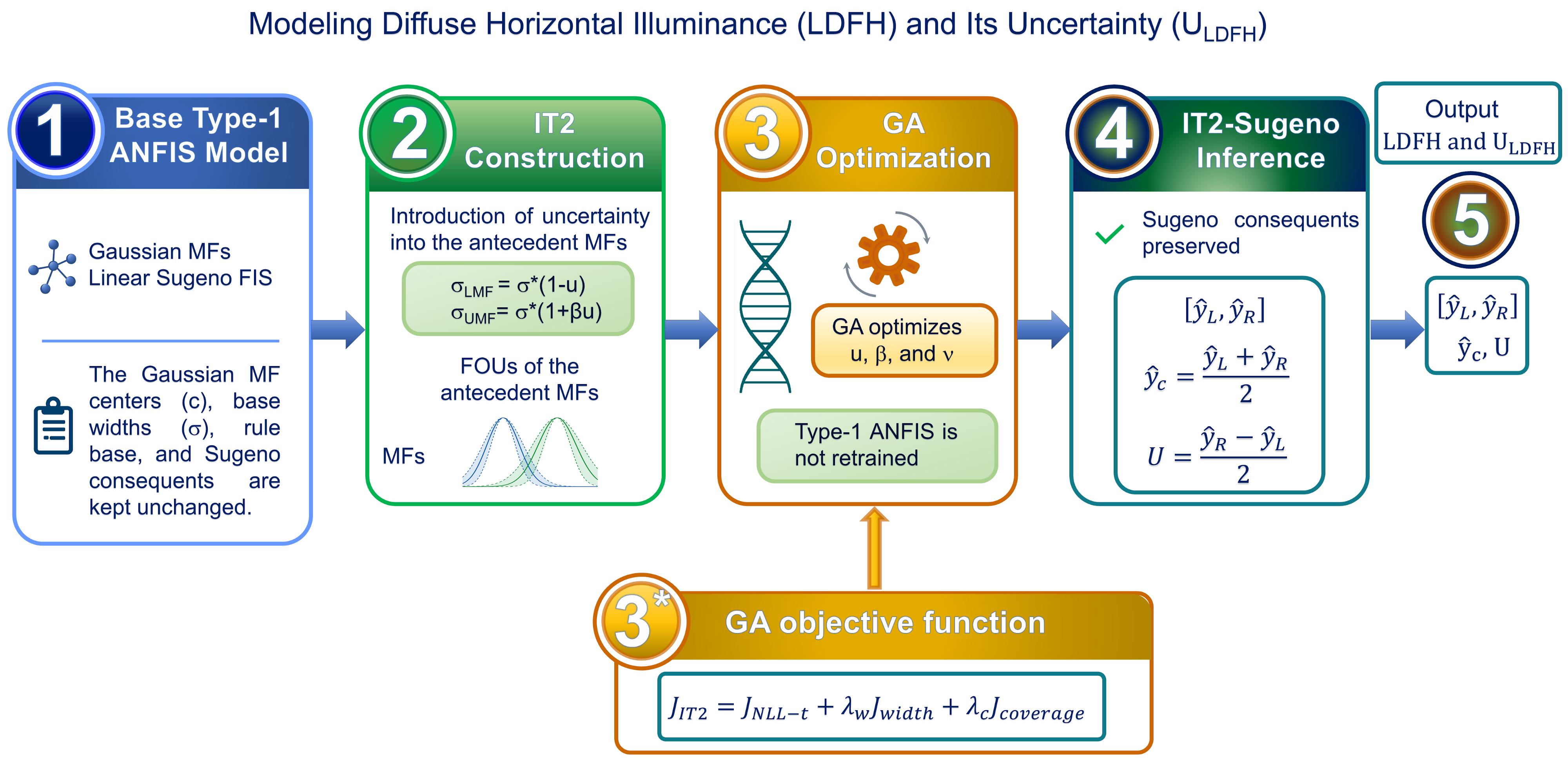
Because daylight illuminance measurements are available at relatively few monitoring stations, luminous-efficacy models have traditionally been used to derive global, direct, and diffuse illuminance data from irradiance measurements [12]. Moreover, recent optimization literature supports the use of evolutionary algorithms for complex engineering problems characterized by large search spaces and multiple competing objectives [13]. This provides a general basis for adopting a GA-based strategy in the present study, where several parameters are optimized by balancing predictive likelihood, interval width, and empirical coverage. However, previous data-driven and neuro-fuzzy approaches have generally focused on illuminance point estimation rather than on the explicit generation and empirical evaluation of predictive intervals for LDFH. Therefore, this study proposes a two-stage neuro-fuzzy framework for the direct estimation and uncertainty quantification of LDFH from DHI, solar altitude, and zenith luminance, combining radiometric, geometric, and sky-photometric information available at comprehensive daylight-monitoring stations. Specifically, LDFH is estimated directly without applying intermediate luminous-efficacy methods, thereby providing a compact and physically interpretable input structure. In the first stage, a first-order Sugeno Type-1 ANFIS with Gaussian membership functions is developed to learn the central nonlinear relationship between the input variables and LDFH. In the second stage, the Type-1 ANFIS is extended to an Interval Type-2 Sugeno system aimed at quantifying the uncertainty associated with the estimates.
The main contributions of this study are as follows:
- LDFH is estimated directly, avoiding intermediate luminous-efficacy conversions and combining radiometric, solar-geometric, and sky-photometric information within a single predictive model.
- A first-order Type-1 Sugeno ANFIS is extended to an Interval Type-2 Sugeno system to provide sample-specific predictive intervals in addition to point estimates of LDFH.
- The Type-1 structure is preserved in the IT2 extension, while uncertainty is introduced into the antecedent membership functions, allowing point estimation and uncertainty quantification to be treated within the same neuro-fuzzy framework.
- Reduced ANFIS configurations are evaluated to quantify the individual contribution of solar geometry and zenith luminance. In particular, a reduced model based only on DHI and sin(α) is also extended to the IT2-Sugeno formulation, providing an alternative when zenith luminance measurements are unavailable.
- Regression models using the same input configurations are included as reference models to assess the added value of the ANFIS approach.
- Independent annual datasets from 2019 to 2023 are used to evaluate interannual model performance and the empirical coverage of the predictive intervals.
These contributions provide a framework for estimating diffuse horizontal illuminance together with its associated uncertainty, while also allowing the effect of input availability on predictive performance to be assessed.
Figure 1 provides a schematic overview of the proposed framework, from the trained Type-1 ANFIS model to the final Interval Type-2 Sugeno prediction. The Type-1 structure is preserved, while uncertainty is introduced into the antecedent membership functions through the construction of footprints of uncertainty (FOUs). The FOU is the region bounded by the lower and upper membership functions and represents the uncertainty associated with the membership grade of each input. Its propagation through the fuzzy inference system results in lower and upper bounds for the predicted LDFH. The FOU parameters, together with the Student-t degrees of freedom, are optimized using the genetic algorithm, while the Type-1 ANFIS rule structure and consequents remain unchanged. In this way, the framework combines point estimation and uncertainty quantification within the same neuro-fuzzy structure.
The rest of the paper is structured as follows. Section 2 introduces the experimental dataset, the filtering procedure, and the selected input and output variables for LDFH estimation. Section 3 describes the proposed Type-1 Sugeno ANFIS model and its Interval Type-2 Sugeno extension optimized by a genetic algorithm. Sections 4 and 5 present and discuss the results, including the performance of the LDFH estimates and the empirical assessment of the predictive intervals, respectively. Finally, the main conclusions and future research directions are presented.
2. Experimental data and methods
This section details the measurement data, predictor selection, and statistical framework employed to build the ANFIS models aimed at estimating diffuse horizontal illuminance and its associated uncertainty.
2.1. Measurement facilities and predictor variables used in the ANFIS models
The experimental dataset was obtained from the Vaulx-en-Velin IDMP station in France, located at 45°46′43′′ N and 4°55′21′′ E. It comprised diffuse horizontal illuminance, diffuse horizontal irradiance, zenith luminance, and atmospheric variables measured at 1 min resolution over the 2019-2024 period. For model development, only the 2024 records were used to train the ANFIS structure. The year 2024 was selected as the development year without applying any criterion based on model performance or data quality. Once the model had been developed using only the 2024 campaign, five additional complete annual measurement campaigns, corresponding to 2019-2023, were selected exclusively for external validation to assess its robustness to interannual variability. These datasets were kept completely separate from model training and parameter selection, ensuring an independent assessment of model performance across different years. Because each validation dataset covers a complete calendar year, the evaluation incorporates seasonal and meteorological variability, allowing model generalization to be assessed across the range of solar and sky conditions occurring throughout the year. Details of the measurement system, including the instrumentation, can be found in the documentation of the ENTPE CIE-IDMP station [14].
Prior to the analysis, the downloaded records were processed according to the CIE [15] quality-control recommendations. The dataset was further refined by discarding invalid samples and removing observations acquired when the solar altitude was lower than 5°.
The explanatory variables included in the correlation analysis of Table 1 were derived from the irradiance measurements and solar-position parameters according to Eqs. (1)-(5). First, the extraterrestrial normal irradiance was calculated from the solar constant corrected for the annual variation in the Sun-Earth distance:
where Isc=1361 W/m2 is the solar constant [16], and
with dn representing the day number. The clearness index
where α is the solar altitude angle. In addition, two sky-condition descriptors proposed by Perez et al. [17] were considered. The sky clearness index was calculated from the diffuse and direct normal irradiance components and the solar zenith angle Z, expressed in radians, as shown in Eq. (4).
The sky brightness index, Δ, was obtained from Eq. (5), where m is the relative optical air mass.
As shown in Table 1, the correlation pattern for diffuse horizontal illuminance (LDFH) highlights the dominant role of the diffuse radiative component and daylight-related sky conditions. Among the analyzed predictors, DHI exhibits a strong positive association with LDFH, confirming that diffuse horizontal irradiance is the main radiometric predictor of diffuse horizontal illuminance. The sine of the solar altitude, sin(α), was also retained because it accounts for the geometric dependence of horizontal daylight quantities on the apparent position of the sun. In addition, zenith luminance was included as a final predictor because it provides direct photometric information on the brightness state of the sky vault, which is especially relevant for diffuse illuminance estimation. Although other variables, such as GHI, BHI, Kt, ε and Δ, among others, were analyzed to characterize the radiative and sky-condition context, they were not incorporated into the final LDFH model. Several of these variables are strongly linked to the same underlying irradiance balance or can be derived from the measured irradiance components, which could introduce redundant information into the ANFIS structure. Therefore, the final input set was restricted to DHI, sin(α), and zenith luminance. This selection preserves the main physical and photometric mechanisms controlling LDFH while keeping the model structure simple and reducing redundancy among predictors. The influence of the selected predictors on model performance is further assessed using reduced-input ANFIS configurations, as discussed in Section 4.
2.2. Statistical metrics for model evaluation
The predictive accuracy of the models was assessed using nRMSE (%), nMBE (%), and nMAE (%). These normalized indicators were adopted as the main error metrics to compare model behavior across the different datasets. Eqs. (6)-(8) define these statistics, where yj is the measured value, ŷj is the corresponding model estimate, ȳ is the mean measured LDFH and n is the number of observations.
Furthermore, the coefficient of determination, (R2), given in Eq. (9) and the Willmott’s index of agreement [18], defined in Eq. (10), were included as complementary goodness-of-fit indicators.
3. Modeling of diffuse horizontal illuminance (LDFH)
This section presents the modeling of the diffuse horizontal illuminance (LDFH) using ANFIS models.
3.1. Type-1 Sugeno ANFIS for LDFH estimation
The estimation of LDFH was carried out using a first-order Sugeno ANFIS. Model initialization was performed in Matlab using the Fuzzy Logic Toolbox™ [19]. Specifically, the initial FIS was obtained with the genfis function by applying grid partitioning to the selected input space. The model included three predictors, namely DHI, sin(α), and zenith luminance, and each input was represented by two Gaussian membership functions which were used to ensure continuous changes in membership degree across neighboring regions of the input space. For an input value x, the membership degree was calculated according to Eq. (11).
In the adopted ANFIS structure, the three-dimensional input domain was partitioned by assigning two fuzzy Gaussian sets to each predictor. The grid-based initialization then formed the rule base by combining the membership functions defined for DHI, sin(α), and zenith luminance. This led to 23=8 first-order Sugeno rules, each one describing a different region of the input domain. The model was trained using all valid records from 2024 for 50 epochs with the hybrid method, which combines backpropagation and least-squares estimation. With this configuration, the model can account for the main changes in LDFH associated with diffuse irradiance, solar altitude, and sky brightness, while keeping the number of model coefficients within a controlled range. The general rule structure is expressed in Eq. (12). If DHI is Ai and sin(α) is Bj and zenith luminance is Cl, then
Here, the coefficients
Equation (14) defines the normalized firing strength of the k-th rule (
The output of the first-order Sugeno FIS [20] was then obtained by aggregating the linear outputs of all rules according to their normalized firing strengths, as shown in Eq. (15). In this expression, (
After the initial Sugeno rule base had been generated, model training was carried out using ANFIS. The learning process adjusted both parts of the fuzzy model: the antecedent membership functions and the linear consequent equations. These parameters were estimated from the 2024 training records according to the adaptive neuro-fuzzy learning method introduced by Jang [21]. Negative output values are not physically admissible for diffuse horizontal illuminance. Therefore, when the ANFIS model produced a negative LDFH estimate, the value was set to zero before computing the final results, as indicated in Eq. (16).
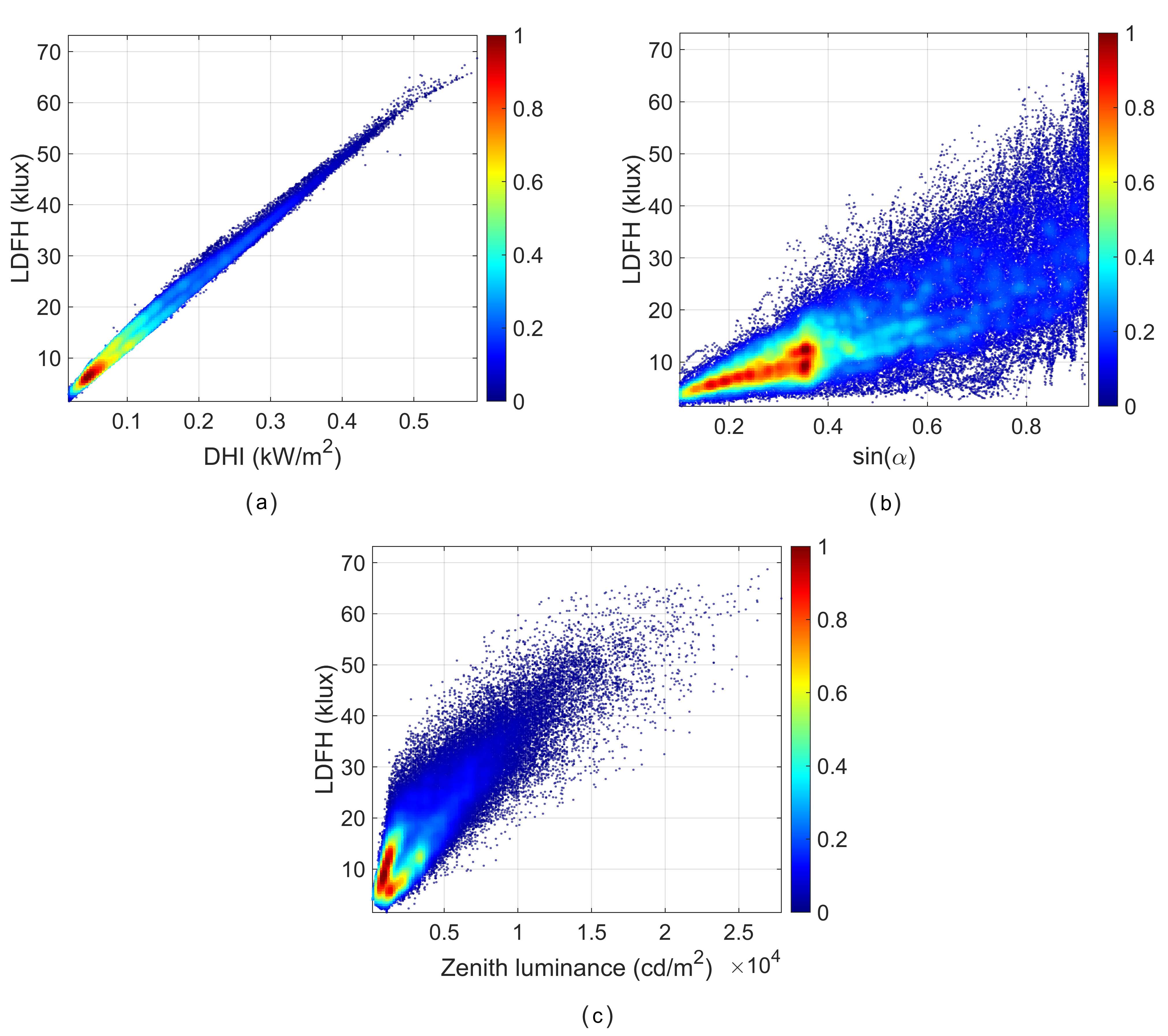
Figure 2(a) shows that DHI has the most direct and nearly linear relationship with LDFH, confirming its role as the main radiometric predictor. However, the relationship between LDFH and sin(α) shown by Figure 2(b) presents a broader distribution, indicating that solar geometry modulates diffuse illuminance but does not explain it by itself. In turn, zenith luminance shows a clear positive association with LDFH, as shown in Figure 2(c), although with greater dispersion than DHI, suggesting that it provides additional photometric information on sky brightness. These patterns support the combined use of DHI, sin(α), and zenith luminance in the complete model. It should also be noted that, before selecting the final input structure, reduced ANFIS models based on subsets of the input variables were evaluated. The results obtained with these reduced configurations were poorer than those of the complete model, which included DHI, sin(α), and zenith luminance. Therefore, DHI, sin(α), and zenith luminance were retained as the final inputs, since this combination outperformed the simpler configurations evaluated in the preliminary comparison, as shown in the next section.
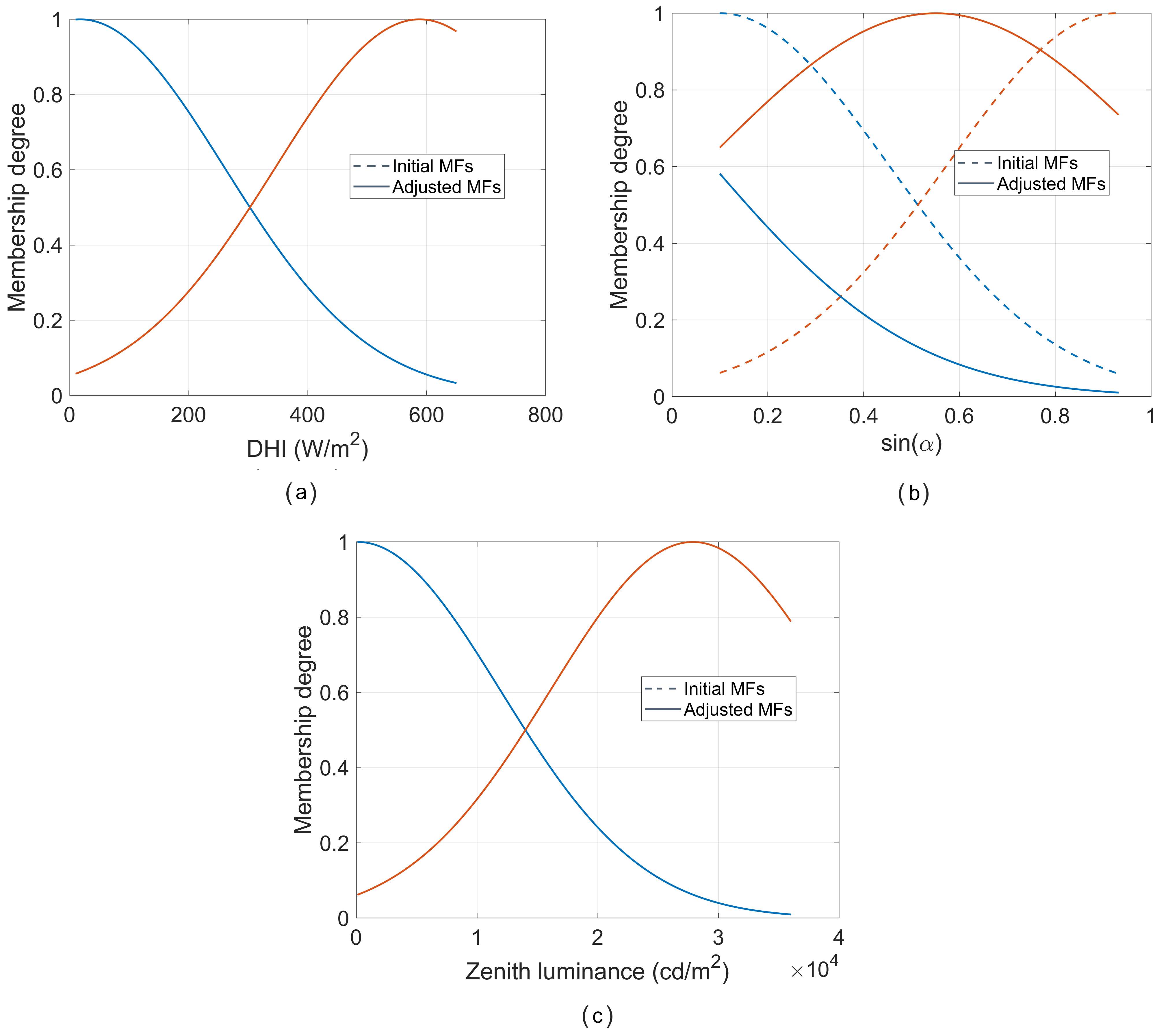
Figure 3 shows the comparison between the initial Gaussian membership functions and those obtained after ANFIS training for the three input variables. For DHI and zenith luminance, the initial and adjusted membership functions remain nearly unchanged after training, indicating that the initial grid-partition structure was already suitable for these two inputs. DHI shows a very direct association with LDFH, while zenith luminance provides a photometric description of the sky-brightness state. In contrast, the variable sin(α) shows a more evident adaptation of its membership functions. After training, the curves associated with this variable are shifted with respect to the initial configuration, reflecting the need to readjust the fuzzy representation of solar geometry.
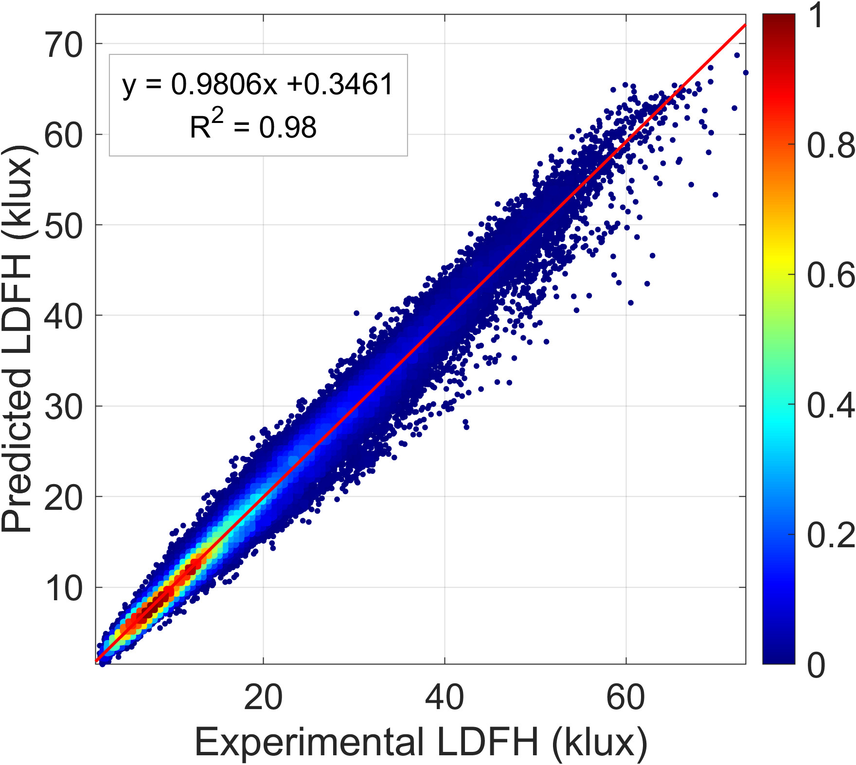
Figure 4 compares the experimental and predicted LDFH values for the 2024 training dataset. The points are closely distributed around the 1:1 line, with a slope of 0.9806 and an R2 of 0.98, indicating strong agreement between the ANFIS estimates and the measured values. A slightly larger dispersion is observed at high LDFH values, although the general trend is well reproduced.
3.2. Interval type-2 Sugeno FIS for LDFH uncertainty modeling
After developing the Type-1 Sugeno ANFIS model, an Interval Type-2 Sugeno FIS [22], [23] was implemented to represent the uncertainty associated with LDFH estimation. For this purpose, the developed Interval Type-2 Sugeno model preserves the rule structure, the centers of the membership functions, and the linear consequents obtained from the Type-1 model. Uncertainty is introduced into the Gaussian antecedents through a footprint of uncertainty, FOU, bounded by a lower membership function, LMF, and an upper membership function, UMF [22], [23]. In this study, the FOU was incorporated by asymmetrically modifying the Gaussian widths, without changing the function centers or the rule base. For each nominal Gaussian function with width (σ), the lower and upper widths were defined as shown in Eqs. (17)-(18), where (u) controls the local amplitude of the FOU, and (β) introduces asymmetry between the lower and upper bounds.
Prediction interval models should provide accurate central estimates while generating intervals that achieve the desired coverage probability without being excessively wide. These three properties are usually quantified through mean squared error (MSE), prediction interval coverage probability (PICP), and prediction interval normalized average width (PINAW), respectively [24], [25], [26]. Previous studies have used these metrics as part of the training loss. For example, [27] combined MSE, PINAW, and a squared penalty on the difference between empirical and target coverage in order to balance central prediction error, coverage, and interval width. The objective adopted here follows this general idea but changes the treatment of the residual error. Instead of using MSE, the residual contribution is formulated as a Student-t negative log-likelihood, where the error is scaled by the uncertainty derived from the IT2-Sugeno interval [28], [29]. The remaining terms control the interval width and penalize failure to reach the target coverage only when the empirical coverage falls below the prescribed level. The Student-t negative log-likelihood is obtained by taking the negative logarithm of the Student-t predictive density, resulting in a residual-dependent logarithmic term together with the scale term and the Gamma-function normalization constants [30].
For each candidate parameter vector
For each candidate solution
In this study, the GA minimizes the objective function given by Eq. (20):
where
The Student-
For the IT2-Sugeno optimization, the loss function used unit weight for the Student-t negative log-likelihood term, with a target coverage of 0.9545. The optimized model was subsequently evaluated using the complete training dataset. As previously mentioned, in this study, the target coverage is set to Ctarget=0.9545, which gives
Thus, the residual term in the Student-t likelihood is evaluated relative to the uncertainty scale implied by the IT2-Sugeno prediction interval, rather than through a fixed variance or a conventional squared-error term. In addition, the width term (
In addition, only failure to reach the target coverage is penalized as shown in Eq. (25). The desired coverage level is set to
| Dataset | Year | nRMSE (%) | nMBE (%) | nMAE (%) | IA | R2 |
|---|---|---|---|---|---|---|
| Train | 2024 | 11.3995 | 0.0000 | 9.1737 | 0.9912 | 0.9657 |
| Test | 2019 | 12.2054 | -0.7491 | 10.3020 | 0.9908 | 0.9631 |
| Test | 2020 | 11.5622 | -0.5909 | 9.7096 | 0.9917 | 0.9671 |
| Test | 2021 | 11.4165 | -1.2199 | 9.4891 | 0.9906 | 0.9631 |
| Test | 2022 | 11.9625 | -3.6178 | 10.0047 | 0.9891 | 0.9574 |
| Test | 2023 | 13.0342 | -2.7643 | 10.1392 | 0.9873 | 0.9516 |
| Dataset | Year | nRMSE (%) | nMBE (%) | nMAE (%) | IA | R2 |
|---|---|---|---|---|---|---|
| Train | 2024 | 10.1842 | 0.0000 | 8.1765 | 0.9930 | 0.9724 |
| Test | 2019 | 10.3974 | -0.5427 | 8.4200 | 0.9932 | 0.9728 |
| Test | 2020 | 9.8398 | -0.6640 | 7.9527 | 0.9939 | 0.9758 |
| Test | 2021 | 10.0617 | -1.1766 | 8.1890 | 0.9927 | 0.9711 |
| Test | 2022 | 10.1236 | -3.2791 | 8.1691 | 0.9921 | 0.9693 |
| Test | 2023 | 11.7047 | -2.9857 | 8.9623 | 0.9897 | 0.9607 |
| Dataset | Year | nRMSE (%) | nMBE (%) | nMAE (%) | IA | R2 |
|---|---|---|---|---|---|---|
| Train | 2024 | 10.4297 | 0.0000 | 7.8260 | 0.9927 | 0.9713 |
| Test | 2019 | 11.5500 | 1.1612 | 9.0185 | 0.9917 | 0.9669 |
| Test | 2020 | 10.6568 | 0.3995 | 8.2473 | 0.9930 | 0.9721 |
| Test | 2021 | 11.0163 | -1.3774 | 8.4364 | 0.9915 | 0.9657 |
| Test | 2022 | 11.4356 | -3.7611 | 8.8361 | 0.9902 | 0.9610 |
| Test | 2023 | 12.1524 | -2.8504 | 8.7682 | 0.9891 | 0.9579 |
Furthermore, the term (
where
Therefore, the GA searches the bounded parameter space of
4. Results and discussion of type-1 Sugeno ANFIS and quadratic regression models
This section presents the results obtained with the ANFIS model for the direct estimation of diffuse horizontal illuminance from the selected input variables. To assess the contribution of each input variable, this section compares the predictive performance of the complete three-input ANFIS model, M3, with that of the reduced configurations M1, using DHI; M21 using DHI and sin(α), and M22 using DHI and zenith luminance. Their performance is evaluated for both the training dataset and the independent validation years. Regression-based models using the same input combinations are also included as baselines to provide a direct reference for the improvements achieved by the ANFIS models.
4.1. Performance of the type-1 Sugeno ANFIS models using reduced sets of input variables
| Dataset | Year | nRMSE (%) | nMBE (%) | nMAE (%) | IA | R2 |
|---|---|---|---|---|---|---|
| Train | 2024 | 8.5467 | 0.0000 | 6.0958 | 0.9951 | 0.9806 |
| Test | 2019 | 9.0869 | 2.1022 | 6.6984 | 0.9948 | 0.9793 |
| Test | 2020 | 8.3676 | 0.8673 | 6.1138 | 0.9956 | 0.9825 |
| Test | 2021 | 9.1788 | -1.7407 | 6.6242 | 0.9940 | 0.9760 |
| Test | 2022 | 9.0774 | -3.4088 | 6.6395 | 0.9937 | 0.9753 |
| Test | 2023 | 10.5903 | -3.4768 | 7.1210 | 0.9916 | 0.9678 |
As indicated previously, the Type-1 ANFIS models were initialized using grid partitioning, with two Gaussian membership functions per input and first-order linear consequents. This configuration resulted in two rules for M1, four for M21 and M22, and eight for M3. All models were trained for 50 epochs using the valid records from 2024 and the hybrid method, which combines backpropagation to adjust the membership-function parameters and least-squares estimation for the consequents.
Table 2, Table 3, and Table 4 show the performance of the three reduced ANFIS models for both the 2024 training dataset and the independent test years 2019-2023. M1, based only on DHI, shows the largest errors, with nRMSE values ranging from 11.40% to 13.03% and nMAE values from 9.17% to 10.30%. The incorporation of sin(α) in M21 consistently improves performance in all years analyzed, reducing nRMSE relative to M1 by 10.7% during training and, on average, by 13.4% over the test years. M21 also achieves the highest IA and R² values among the reduced models in all test datasets, with nRMSE values ranging from 9.84% to 11.70%. The incorporation of zenith luminance in M22 also improves the results relative to M1, although to a lesser extent, with an average nRMSE reduction of 5.6% over the independent years. M22 nevertheless shows slightly lower nMAE values than M21 during training and in 2023. Taken together, these results show that both additional variables provide useful information compared with the use of DHI alone, but that, when considered individually, sin(α) provides a more consistent improvement in predictive performance than zenith luminance.
4.2. Performance of the type-1 Sugeno ANFIS model using the full set of input variables
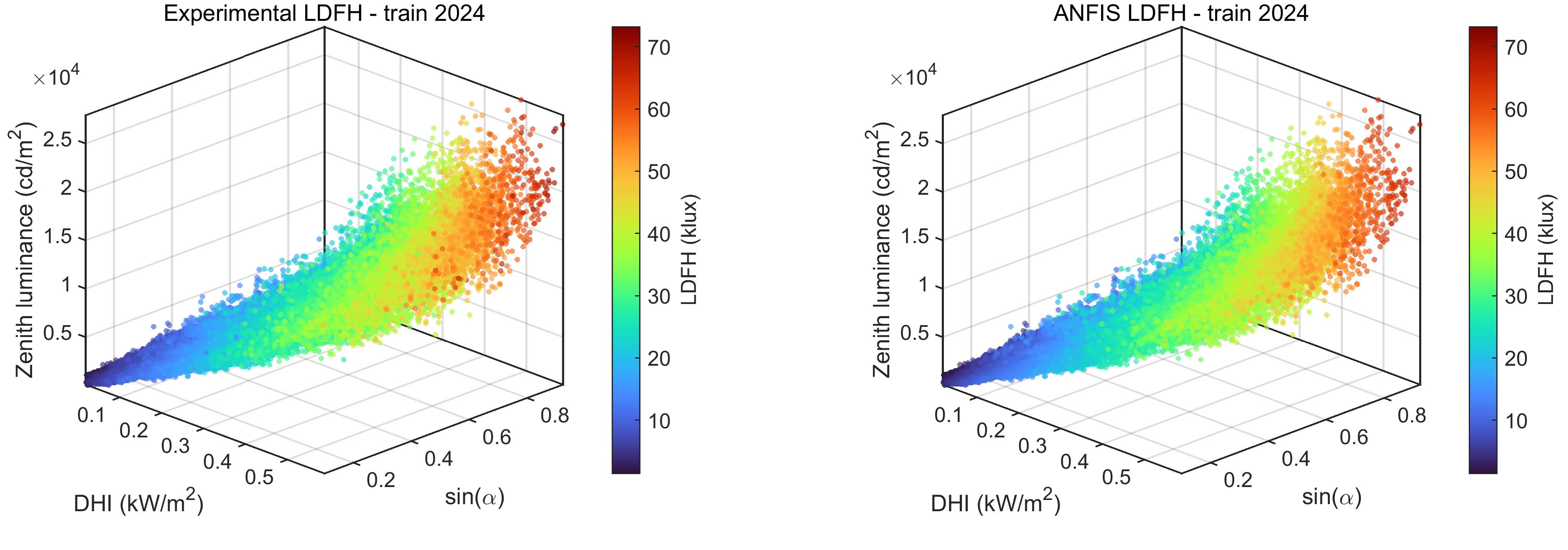
Figure 5 shows the three-dimensional distribution of the experimental LDFH and the LDFH estimated by the ANFIS model for the 2024 training dataset. In both cases, the x-axis represents DHI, the y-axis represents
The LDFH distribution shows that it is mainly controlled by DHI. The lowest LDFH values are concentrated at low DHI, especially below approximately 0.05-0.10 kW m−2, where the color scale remains in the lower range. As DHI increases, LDFH increases progressively, reaching the highest values in the upper DHI region, around 0.3-0.5 kW m−2. These maximum LDFH values appear mainly when zenith luminance is also high, indicating that large diffuse illuminance is associated with the combined effect of high diffuse irradiance and strong sky brightness near the zenith. Figure 5 shows that maximum LDFH occurs under conditions of simultaneously high DHI, high zenith luminance, and moderate-to-high solar elevation.
Table 5 shows that the Type-1 Sugeno ANFIS model for the direct estimation of LDFH achieves, for the training dataset, an nRMSE of 8.55%, an nMAE of 6.10%, an IA of 0.9951, and an R2 of 0.9806, indicating a good fit to the training data. For the independent test years 2019-2023, the performance remains stable, with nRMSE values between 8.37% and 10.59%, IA values above 0.991, and R2 values higher than 0.967. Although these results confirm the suitability of the Type-1 ANFIS model as a deterministic estimator, they only quantify point-prediction accuracy and do not provide information about the uncertainty associated with each estimate, which motivates the use of an Interval Type-2 Sugeno model. In practical terms, the training nRMSE of 8.55% for 2024 indicates that the root mean square error corresponds to approximately 8.55% of the mean measured LDFH for the dataset. This value should therefore be interpreted as an overall measure of prediction error relative to the mean diffuse illuminance level, rather than as an 8.55% error for each individual observation. Together with the low nMBE and the high IA and R² values, it indicates that the model adequately reproduces both the magnitude and variability of LDFH.
Compared with the reduced models, the full M3 model shows the best performance across all datasets analyzed. For the 2024 training dataset, M3 reduces nRMSE to 8.55%, compared with 11.40% for M1, 10.18% for M21, and 10.43% for M22, corresponding to reductions of 25.0%, 16.1%, and 18.1%, respectively. This improvement is maintained over the independent test years: the mean nRMSE of M3 is 9.26%, compared with 12.04% for M1, 10.43% for M21, and 11.36% for M22. Thus, relative to the reduced models, M3 decreases the mean nRMSE over the test years by approximately 23.1% compared with M1, 11.2% compared with M21, and 18.5% compared with M22. The same pattern is observed for nMAE, with mean reductions over the test years of 33.1%, 20.4%, and 23.3%, respectively. In addition, M3 consistently achieves higher IA and R² values. These results show that, although DHI is the main predictor and the individual incorporation of either sin(α) or zenith luminance improves the estimation, the combined use of both additional variables provides a further and consistent improvement, thereby justifying the increased complexity of the M3 model. However, the M21 model could also be used when zenith luminance measurements are not available.
4.3. Performance of the regression-based models
To provide a reference for evaluating the added value of the ANFIS approach, regression-based models were also developed using the same combinations of input variables considered in the reduced and full ANFIS models. Thus, M1 uses only DHI, M21 combines DHI and sin(α), M22 combines DHI and zenith luminance, and M3 incorporates all three input variables. All regression models were fitted using the 2024 training dataset and subsequently evaluated for the independent test years 2019-2023 using the same performance metrics employed for the ANFIS models.
The regression baselines consisted of quadratic regression models fitted by ordinary least squares with an intercept. They included linear terms, squared terms, and, where applicable, all two-factor interactions. The resulting M1, M21, M22, and M3 models are shown in Eqs. (28)-(31).
As can be seen in Table 6, Table 7, Table 8, and Table 9, the four quadratic regression models show improved performance as additional variables are incorporated. M1, based only on DHI, presents the largest errors, with a mean nRMSE of 12.08% and a mean nMAE of 9.95% over the independent test years. The incorporation of sin(α) in M21 produces a clear and consistent improvement, reducing these mean values to 10.60% and 8.49%, respectively, corresponding to reductions of 12.2% in nRMSE and 14.7% in nMAE relative to M1. M22, which incorporates zenith luminance, also improves upon M1, although to a lesser extent, with a mean nRMSE of 11.69% and a mean nMAE of 9.09%. Therefore, when considered individually, sin(α) provides a greater improvement than zenith luminance. The best performance is obtained with M3, which combines all three input variables, with mean nRMSE and nMAE values of 9.84% and 7.33%, respectively. Compared with M1, these values represent reductions of 18.6% and 26.3%, while relative to M21, the additional reductions are 7.2% and 13.7%. M3 also generally presents the highest IA and R² values. Taken together, the results show that the combined use of DHI, sin(α), and zenith luminance provides the best performance among the quadratic regression models, although the largest individual additional contribution relative to DHI comes from sin(α).
| Dataset | Year | nRMSE (%) | nMBE (%) | nMAE (%) | IA | R2 |
|---|---|---|---|---|---|---|
| Train | 2024 | 11.4217 | 0.0000 | 9.1738 | 0.9912 | 0.9656 |
| Test | 2019 | 12.2700 | -0.7411 | 10.3387 | 0.9906 | 0.9627 |
| Test | 2020 | 11.5856 | -0.5578 | 9.7205 | 0.9917 | 0.9670 |
| Test | 2021 | 11.4856 | -1.2608 | 9.5294 | 0.9905 | 0.9627 |
| Test | 2022 | 12.0021 | -3.6198 | 9.9961 | 0.9890 | 0.9571 |
| Test | 2023 | 13.0652 | -2.7767 | 10.1572 | 0.9873 | 0.9514 |
| Dataset | Year | nRMSE (%) | nMBE (%) | nMAE (%) | IA | R2 |
|---|---|---|---|---|---|---|
| Train | 2024 | 10.3489 | 0.0000 | 8.3159 | 0.9927 | 0.9715 |
| Test | 2019 | 10.6398 | -0.4227 | 8.6177 | 0.9928 | 0.9716 |
| Test | 2020 | 9.9831 | -0.5551 | 8.0828 | 0.9937 | 0.9751 |
| Test | 2021 | 10.2733 | -1.1399 | 8.4165 | 0.9923 | 0.9699 |
| Test | 2022 | 10.2618 | -3.2270 | 8.2380 | 0.9919 | 0.9684 |
| Test | 2023 | 11.8632 | -3.0746 | 9.0935 | 0.9894 | 0.9596 |
| Dataset | Year | nRMSE (%) | nMBE (%) | nMAE (%) | IA | R2 |
|---|---|---|---|---|---|---|
| Train | 2024 | 10.8069 | 0.0000 | 8.2835 | 0.9921 | 0.9692 |
| Test | 2019 | 11.8626 | 0.6607 | 9.5777 | 0.9913 | 0.9651 |
| Test | 2020 | 11.0392 | 0.1949 | 8.8336 | 0.9925 | 0.9700 |
| Test | 2021 | 11.5378 | -1.3969 | 8.8494 | 0.9906 | 0.9623 |
| Test | 2022 | 11.6809 | -3.9362 | 9.1503 | 0.9897 | 0.9594 |
| Test | 2023 | 12.3192 | -2.9337 | 9.0361 | 0.9888 | 0.9568 |
| Dataset | Year | nRMSE (%) | nMBE (%) | nMAE (%) | IA | R2 |
|---|---|---|---|---|---|---|
| Train | 2024 | 9.1677 | 0.0000 | 6.8297 | 0.9943 | 0.9777 |
| Test | 2019 | 9.8792 | 1.8896 | 7.5889 | 0.9939 | 0.9755 |
| Test | 2020 | 9.0311 | 0.6600 | 6.9174 | 0.9949 | 0.9797 |
| Test | 2021 | 9.7628 | -1.9513 | 7.2949 | 0.9932 | 0.9728 |
| Test | 2022 | 9.5767 | -3.9386 | 7.1686 | 0.9930 | 0.9725 |
| Test | 2023 | 10.9305 | -3.8695 | 7.6717 | 0.9911 | 0.9657 |
The comparison between the ANFIS models and the quadratic regressions shows that the largest difference is observed for M3, for which ANFIS reduces the mean nRMSE from 9.84% to 9.26%, a reduction of approximately 5.9%, and the mean nMAE from 7.33% to 6.64%, a reduction of approximately 9.4%. For the M3 training dataset, the reductions reach 6.8% in nRMSE and 10.7% in nMAE, highlighting the greater ability of ANFIS to represent the nonlinear relationships among DHI, sin(α), zenith luminance, and LDFH. The Type-1 ANFIS structure also provides the basis for the Interval Type-2 extension used in this study, which generates sample-specific predictive intervals that can be evaluated in terms of their empirical coverage and width.
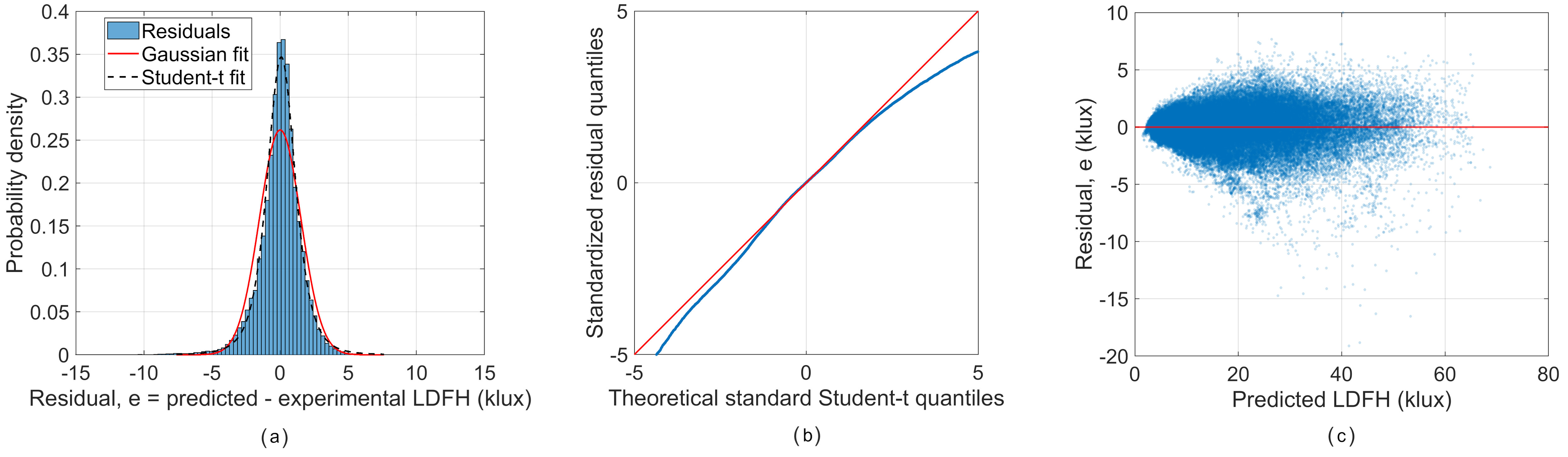
Figure 6 analyzes the residual behavior of the Type-1 ANFIS model for LDFH using the 2024 training dataset. The residual histogram in Figure 6(a) shows that most errors are centered around zero, indicating no substantial systematic bias in the deterministic ANFIS predictions. However, the residual distribution departs from a Gaussian distribution, with a sharper central peak and heavier tails than the Gaussian fit. Likewise, Figure 6(b) compares the empirical quantiles of the standardized residuals with the theoretical standard Student-t quantiles and shows good agreement across the central quantiles, although deviations remain in the distribution tails. Figure 6(c) provides a complementary representation of the residuals as a function of the predicted LDFH, showing an increase in residual dispersion at higher predicted illuminance levels. From a modeling perspective, Figure 6(a) indicates that relatively large prediction errors occur more frequently than would be expected under a Gaussian assumption. This represents a limitation of a purely Gaussian description of the residual uncertainty and supports the use of the Student-t likelihood in the IT2 optimization because of its greater robustness to heavy-tailed errors. However, the remaining deviations in the tails of the Student-t Q-Q plot also indicate that this distribution does not perfectly reproduce all residual behavior.
| Input | MF |
|
|
|
|
|
|---|---|---|---|---|---|---|
| DHI | mf1 | 242.07 | 18.00 | 0.073 | 224.46 | 260.47 |
| mf2 | 242.08 | 587.98 | 0.039 | 232.60 | 251.99 | |
| Zenith luminance | mf1 | 11780.09 | 140.00 | 0.003 | 11739.65 | 11822.37 |
| mf2 | 11780.09 | 27880.00 | 0.001 | 11768.21 | 11792.52 | |
|
|
mf1 | 0.42 | -0.34 | 0.001 | 0.42 | 0.42 |
| mf2 | 0.49 | 0.55 | 0.072 | 0.45 | 0.52 |
| Dataset | Year | N | Coverage (%) |
Mean uncertainty (klux) |
Median uncertainty (klux) |
|---|---|---|---|---|---|
| Train | 2024 | 95438 | 95.10 | 4.06 | 3.89 |
| Test | 2019 | 141970 | 95.69 | 3.59 | 3.33 |
| Test | 2020 | 126344 | 96.24 | 3.80 | 3.54 |
| Test | 2021 | 120688 | 94.43 | 4.07 | 3.79 |
| Test | 2022 | 118994 | 94.76 | 3.90 | 3.57 |
| Test | 2023 | 120799 | 93.00 | 4.14 | 3.88 |
5. Results and discussion of the interval type-2 Sugeno FIS for uncertainty estimation
This section analyzes the uncertainty provided by the IT2-Sugeno formulation. The analysis first focuses on the full-input model M3, which uses DHI, sin(α), and zenith luminance, and subsequently considers the reduced model M21, based only on DHI and sin(α). The latter allows the predictive uncertainty performance of the proposed approach to be assessed when zenith luminance measurements are unavailable, while also enabling direct comparison with the full-input model.
5.1. Full-input IT2-Sugeno model (M3)
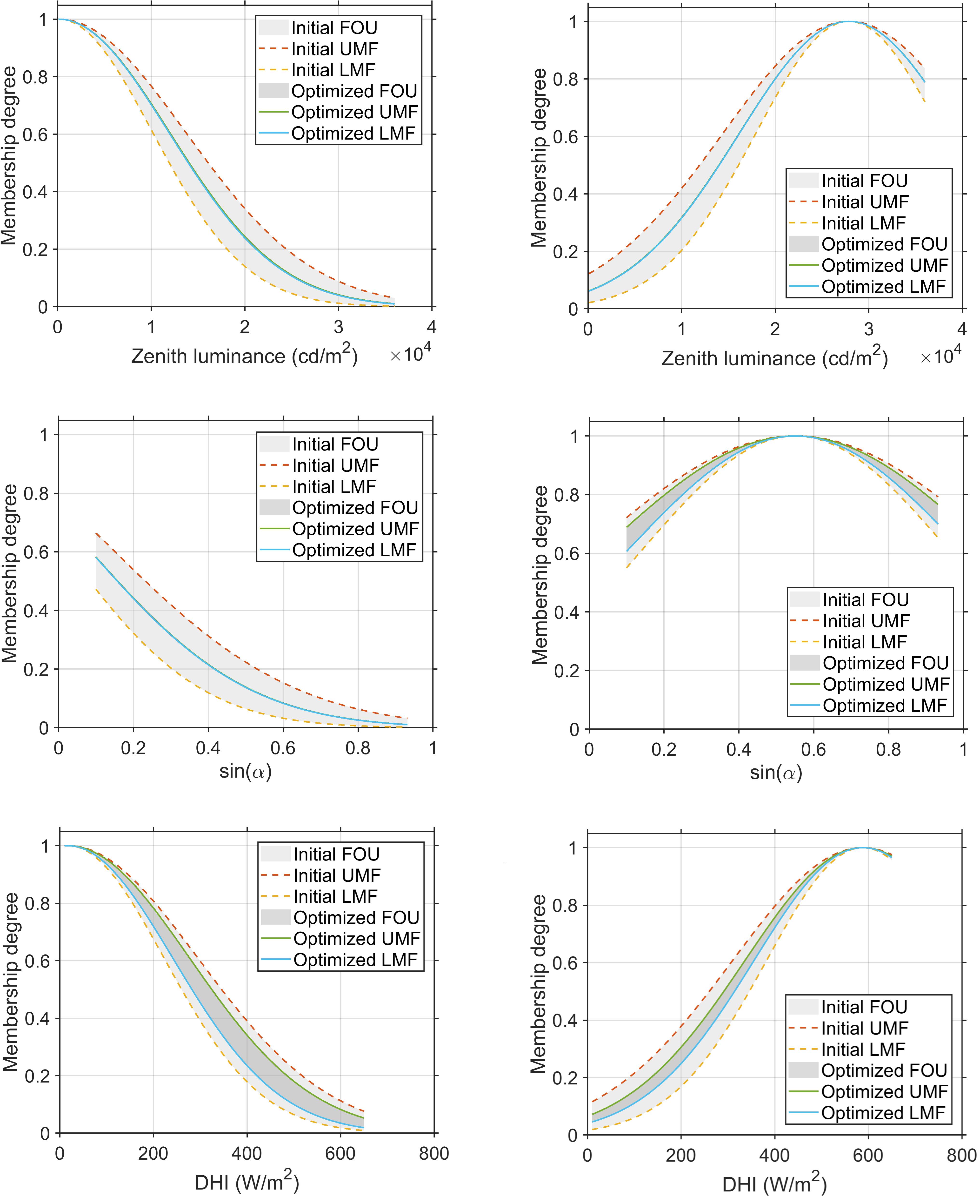
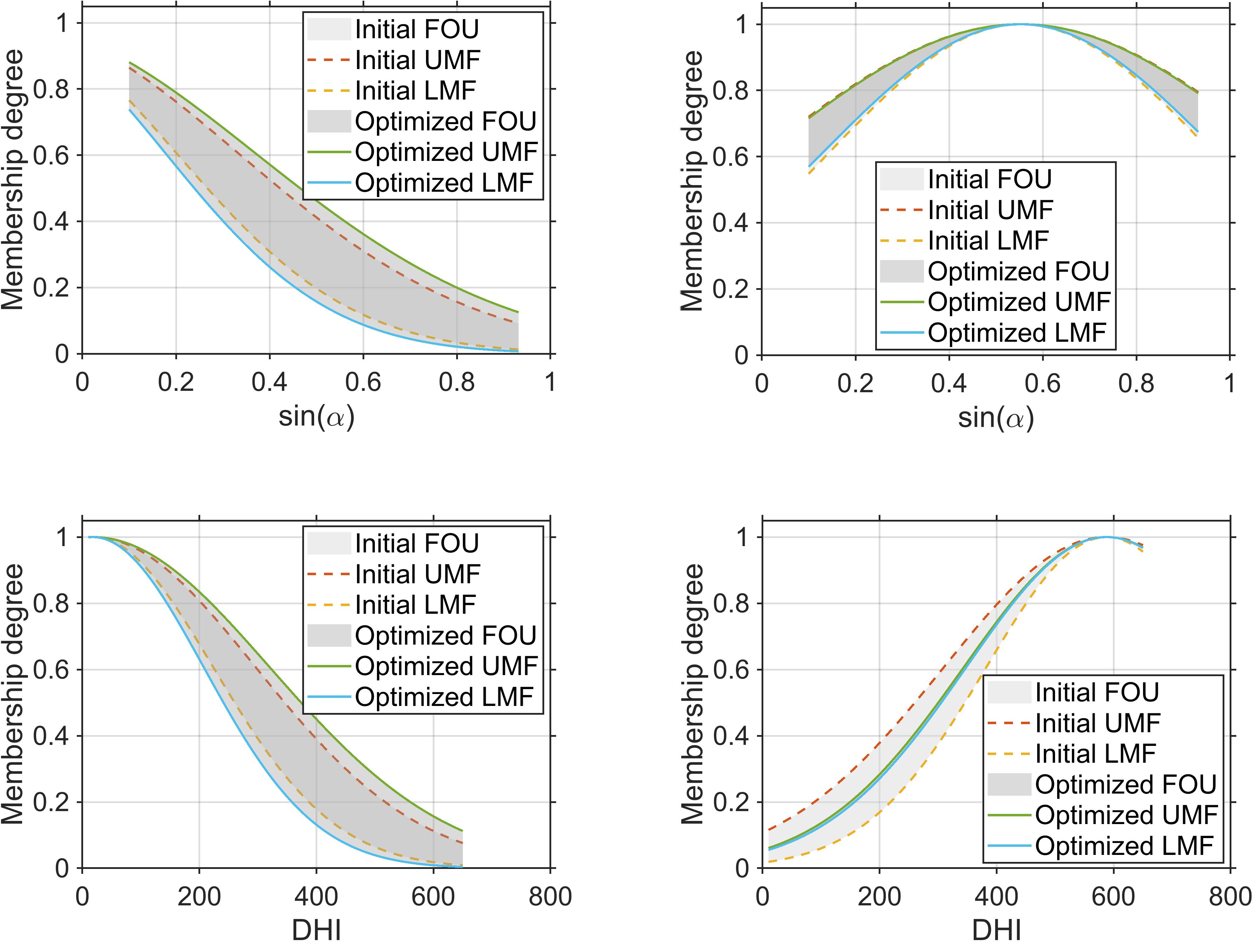
Figure 7 compares the initial and GA-optimized FOUs of the antecedent membership functions in the IT2-Sugeno model proposed for LDFH estimation. The initial FOUs are constructed from the antecedent membership functions of the previously trained Type-1 ANFIS model. The final FOUs are obtained by optimizing the uncertainty parameters through the genetic algorithm, using the proposed loss function as the optimization criterion.
As can be observed in Figure 7, the optimized FOUs introduce different uncertainty levels across the input variables and membership functions, with larger or smaller expansions reflecting the uncertainty assigned to each antecedent membership function during optimization. The membership function centers are kept fixed from the trained Type-1 ANFIS in order to preserve the learned fuzzy partition, rules, and nominal input-output relationship. Thus, the GA optimization adjusts the FOU parameters without retraining the antecedent structure or the consequents. Uncertainty is incorporated at the antecedent level, allowing the IT2-Sugeno model to generate prediction intervals while retaining the structural basis of the Type-1 ANFIS model.
In addition, Table 10 reports the GA-optimized FOU parameters of the antecedent membership functions used in the LDFH IT2-Sugeno model. The centers and nominal Gaussian widths of the underlying Type-1 membership functions remain unchanged after optimization, thereby preserving the fuzzy partition learned by the Type-1 ANFIS. The GA adjusts the FOU parameters (u and β), together with the Student-t degrees of freedom parameter (ν). The optimized results show that the largest uncertainty amplitudes are associated with the DHI membership functions and the second membership function of sin(α).
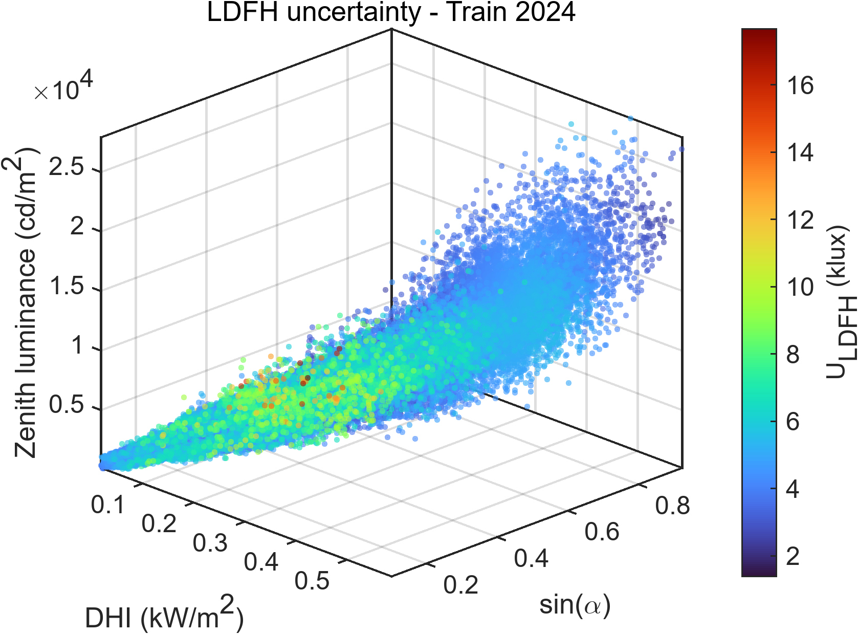
Figure 8 shows the spatial distribution of the uncertainty estimated by the IT2-Sugeno model for LDFH over the 2024 training dataset. The highest uncertainty values are mainly concentrated at low solar elevation and at low to moderate zenith luminance levels, whereas the uncertainty tends to decrease at higher sin(α) and higher zenith luminance. This pattern is consistent with the three-dimensional LDFH distributions shown previously for the measured and ANFIS-estimated values. As shown in Figure 5, the largest LDFH values occur mainly for high DHI, high sin(α), and high zenith luminance. However, Figure 8 shows that these high-illuminance regions are not necessarily associated with the largest predictive uncertainty. Therefore, the IT2-Sugeno interval model does not merely increase the interval width as LDFH increases. Instead, it captures the local uncertainty structure of the input-output relationship, with wider intervals in the lower-solar-elevation and lower-zenith-luminance regions.
Table 11 reports the empirical coverage and uncertainty of the IT2-Sugeno interval model for LDFH. The number of samples
A similar behavior is observed in the external validation years 2019 and 2020, where the empirical coverage is 95.69% and 96.24%, respectively. The years 2021 and 2022 also remain close to the target level, with coverages of 94.43% and 94.76%. The mean uncertainty remains relatively stable throughout the years analyzed, ranging from 3.59 to 4.14 klux. The median values are slightly lower than the corresponding means, which suggests that most samples are associated with moderate interval widths, while a smaller fraction of observations leads to wider intervals.
The lowest coverage is obtained in 2023 (93.00%), which also presents the largest mean uncertainty (4.14 klux), indicating that the lower coverage is not simply due to narrower prediction intervals. In addition, 2023 shows the highest nRMSE (10.59%) and the most negative nMBE (-3.48%) among the independent test years. Since the model was trained using only the 2024 dataset and subsequently applied without retraining to each independent year, these differences may reflect interannual variations in the relationship between the input variables and LDFH. Such variations could therefore contribute to the lower coverage observed in 2023.
Table 12 presents selected examples from the 2024 training dataset to illustrate the behavior of the proposed model. The corresponding 95.45% nominal predictive intervals are also reported as [ŷL, ŷR]95.45%. The IT2-Sugeno central estimates remain close to the Type-1 ANFIS outputs, as expected, because the interval extension preserves the rule base, consequent parameters, membership-function centers, and initial Gaussian widths of the original ANFIS model. Furthermore, the predicted values are close to the corresponding experimental LDFH values. The uncertainty is introduced through the footprint of uncertainty associated with the antecedent membership functions. The selected examples show that the proposed model provides both direct LDFH estimates and sample-specific predictive intervals using DHI, zenith luminance, and
|
|
Zenith luminance (cd/m2) |
|
|
|
|
|
|---|---|---|---|---|---|---|
| 35 | 1814 | 0.429 | 4653 | 4268 | 4204 | [2087; 6322] |
| 43 | 550 | 0.191 | 6893 | 6872 | 6682 | [3082; 10283] |
| 55 | 2199 | 0.347 | 6735 | 6464 | 6405 | [3030; 9781] |
| 68 | 1034 | 0.451 | 12719 | 11190 | 11113 | [9129; 13096] |
| 77 | 2751 | 0.360 | 9097 | 9013 | 8978 | [4888; 13067] |
| . | . | . | . | . | ||
| . | . | . | . | . | ||
| . | . | . | . | . | ||
| 102 | 3994 | 0.503 | 11580 | 12158 | 12155 | [8700; 15610] |
| 195 | 5549 | 0.828 | 23570 | 26100 | 25931 | [22162; 29700] |
| 264 | 3994 | 0.745 | 32199 | 33406 | 33238 | [28988; 37489] |
| 286 | 8510 | 0.712 | 33060 | 34657 | 34511 | [29192; 39831] |
| 356 | 16640 | 0.884 | 42647 | 45028 | 44977 | [40749; 49205] |
|
|
|
|
|
|
|
|
|---|---|---|---|---|---|---|
| DHI | mf1 | 242.08 | 17.99 | 0.217 | 189.54 | 302.32 |
| mf2 | 242.08 | 587.97 | 0.008 | 240.05 | 244.4 | |
|
|
mf1 | 0.44 | -0.17 | 0.203 | 0.35 | 0.54 |
| mf2 | 0.49 | 0.55 | 0.122 | 0.43 | 0.55 |
| Model | Inputs | nRMSE (%) | nMAE (%) | Coverage (%) | Mean uncertainty (klux) |
|---|---|---|---|---|---|
| M21 | DHI + sin(α) | 11.59 | 9.01 | 95.74 | 4.48 |
| M3 | DHI + sin(α) + zenith luminance | 9.33 | 6.71 | 94.82 | 3.90 |
|
|
|
|
|
|
|
|---|---|---|---|---|---|
| 35 | 0.429 | 4653 | 5894 | 6305 | [2741; 9869] |
| 43 | 0.191 | 6893 | 5860 | 5573 | [2117; 9029] |
| 55 | 0.347 | 6735 | 7890 | 8280 | [4958; 11602] |
| 68 | 0.451 | 12719 | 9978 | 10317 | [6727; 13908] |
| 77 | 0.36 | 9097 | 10433 | 10557 | [6946; 14167] |
| . | . | . | . | . | |
| . | . | . | . | . | |
| . | . | . | . | . | |
| 102 | 0.503 | 11580 | 14140 | 14305 | [10708; 17902] |
| 195 | 0.828 | 23570 | 26361 | 25824 | [23370; 28278] |
| 264 | 0.745 | 32199 | 32702 | 31872 | [24850; 38893] |
| 286 | 0.712 | 33060 | 34714 | 33317 | [23806; 42828] |
| 356 | 0.884 | 42647 | 43978 | 45208 | [29670; 60747] |
5.2. Reduced-input IT2-Sugeno model (M21)
To assess whether uncertainty can also be quantified when zenith luminance measurements are unavailable, the same IT2-Sugeno formulation and GA optimization procedure were applied to the reduced M21 model, which uses only DHI and sin(α) as inputs. Since the methodology and optimization settings are identical to those described for M3, only the resulting FOU structure and uncertainty are discussed here.
Table 13 shows the optimized parameters of the reduced M21 model, which uses only DHI and sin(α), and may therefore be of interest for stations where zenith luminance measurements are not available.
Figure 9 shows that, as in the full M3 model, the nonuniform redistribution of uncertainty indicates that the optimization does not simply increase the uncertainty of the reduced model globally, but rather distributes it selectively across different regions of the input space according to the predictive-uncertainty patterns identified during optimization.
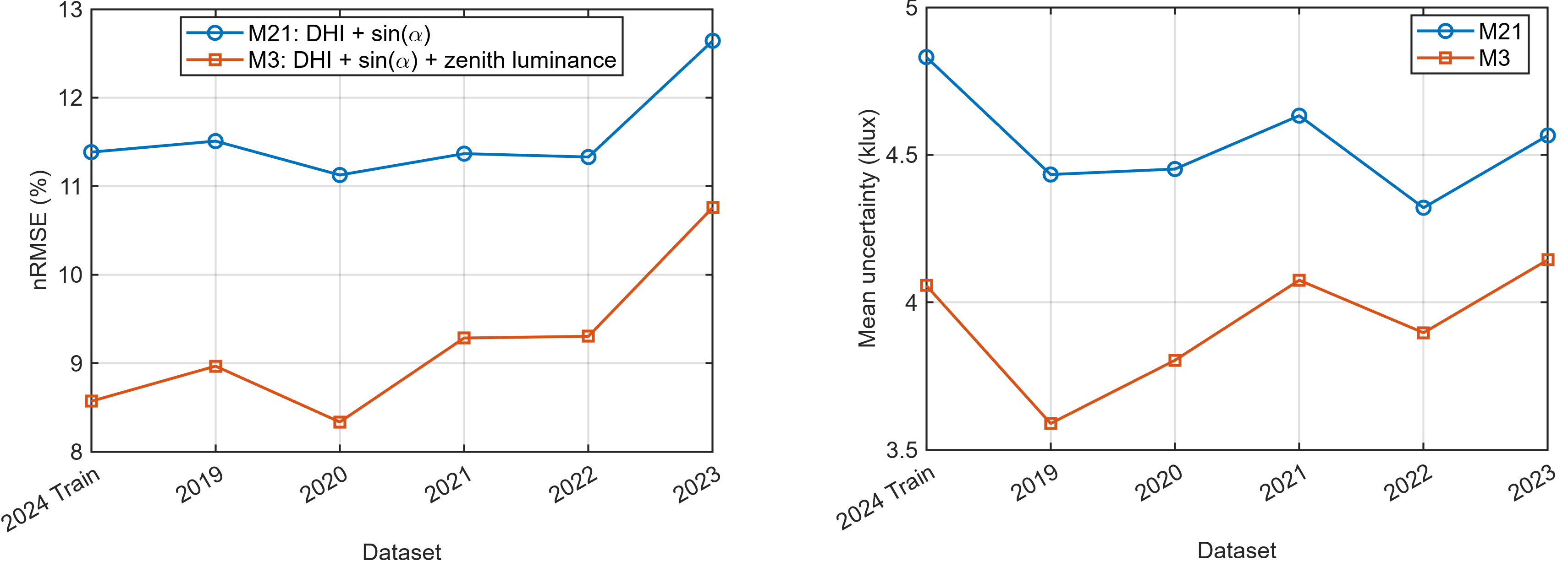
As shown in Table 14, over the five independent test years (2019-2023), the reduced M21 IT2-Sugeno model yielded mean nRMSE and nMAE values of 11.59% and 9.01%, respectively, compared with 9.33% and 6.71% for the full M3 model. These nRMSE and nMAE values correspond to the IT2-Sugeno central predictions. Each reported mean is the arithmetic mean of the corresponding annual values for the five independent test years. Thus, removing zenith luminance increased the mean nRMSE by 24.3% and the mean nMAE by 34.4%. Despite this reduction in point-estimation accuracy, M21 maintained a mean empirical coverage of 95.74%, compared with 94.82% for M3. The coverage obtained with M21 is very close to the nominal target of 95.45%, indicating that the proposed optimization procedure effectively adjusts the FOU to achieve a coverage level close to the prescribed target even when less input information is available. However, this is achieved by widening the prediction intervals, rather than by improving the underlying point-estimation accuracy. Accordingly, the uncertainty increased from 3.90 klux for M3 to 4.48 klux for M21, corresponding to an increase of 14.8%. These results indicate that zenith luminance improves predictive accuracy and reduces uncertainty, whereas the reduced M21 formulation remains a practical alternative for stations where zenith luminance measurements are unavailable, with the comparison against M3 quantifying the corresponding loss in point-estimation accuracy and interval precision. Similarly, Figure 10 shows that the full M3 model consistently outperforms the reduced M21 model in both predictive accuracy and uncertainty. For all independent test years, M3 yields lower nRMSE values and narrower prediction intervals.
A comparison of Table 12 and Table 15 shows the effect of removing zenith luminance on both point estimation and predictive uncertainty for the same selected data points. The full M3 model provides estimates closer to the experimental LDFH values in most the examples shown. Nevertheless, the experimental values remain within the 95.45% predictive intervals generated by M21 in all cases, showing that the reduced model still provides intervals that contain the experimental values for these selected examples despite the loss of one input variable. This is achieved, however, through generally less precise uncertainty characterization, with wider intervals in some cases, particularly for high-illuminance conditions. For the selected examples, the mean interval width increases from 7.24 klux for M3 to 11.13 klux for M21. These results illustrate how the proposed IT2 optimization compensates for the reduced input information by adapting the FOU and, when necessary, widening the predictive intervals to maintain coverage close to the prescribed target.
6. Conclusions
This study addressed the direct estimation of diffuse horizontal illuminance, LDFH, a relevant variable for daylight availability assessment, daylighting design, energy-efficient building analysis, and intelligent lighting-control applications. Since diffuse horizontal illuminance measurements are not always available in experimental daylight databases, the proposed approach provides both predicted LDFH values and prediction intervals associated with each estimate. The methodology first uses a Type-1 Sugeno ANFIS to estimate LDFH and then extends it to a GA-optimized Interval Type-2 Sugeno model to obtain predictive intervals. The M3 model, which uses DHI, sin(α), and zenith luminance as input variables, is proposed as the preferred configuration because it provides the best predictive performance among the evaluated configurations. In addition, the reduced M21 model, based only on DHI and sin(α), could be employed as an alternative for stations where zenith luminance measurements are unavailable.
The Type-1 Sugeno ANFIS model” with “The full-input Type-1 Sugeno ANFIS model (M3) with Gaussian membership functions provided accurate LDFH estimates. The model was trained with the 2024 dataset and evaluated in independent test years from 2019 to 2023. In the training dataset, the Type-1 ANFIS achieved an nRMSE of 8.55%, an
Furthermore, the Interval Type-2 Sugeno extension added uncertainty information to the Type-1 ANFIS estimates. The rule base, consequent parameters, membership-function centers, and initial Gaussian widths were kept unchanged from the Type-1 ANFIS. Uncertainty was introduced through asymmetric footprints of uncertainty in the antecedent membership functions, with the FOU parameters optimized using a genetic algorithm. This formulation allowed the model to produce sample-specific predictive intervals without replacing the original neuro-fuzzy estimation structure.
For a target coverage probability of 95.45%, the GA-optimized IT2-Sugeno model achieved an empirical coverage of 95.10% in the 2024 training dataset, with a mean expanded uncertainty (U) of 4.06 klux. In the independent test years, the empirical coverage ranged from 93.00% to 96.24%, while the mean U remained between 3.59 and 4.14 klux. These results show that the proposed interval model provides relatively stable uncertainty levels across different years. The lowest coverage was obtained in 2023, although the mean uncertainty remained within the same range as the other years, suggesting that the lower coverage may be associated with interannual changes in the residual behavior rather than simply with insufficient interval width.
At the study site, the results support the proposed method for estimating LDFH and quantifying sample-specific predictive uncertainty. These intervals provide additional information that may support daylight-availability and lighting-control studies.
The present study was developed using data from a single monitoring station and one training year, although its performance was evaluated over five independent annual datasets. Future research should extend the evaluation to other stations and climatic conditions, examine the use of predictive intervals in practical daylight applications, and compare alternative uncertainty-quantification methodologies in terms of their ability to provide reliable uncertainty intervals.
Acknowledgement
The author gratefully acknowledges Dr. Dominique Dumortier from ENTPE (France) for providing access to the experimental data used in this study.
Data availability statement
Access to the experimental data supporting the findings of this study was provided by Dr. Dominique Dumortier from ENTPE (France).
Funding
This work received no external funding.
Contributions
MIDV: Conceptualization, Formal analysis, Methodology, Software, Supervision, Validation, Visualization, Writing-original draft, Writing-review & editing.
Declaration of competing interest
The author declares no conflicts of interest.
Disclaimer/Publisher’s Note: The statements, opinions and data contained in all publications are solely those of the individual author(s) and contributor(s) and not of Solarlits and/or the editor(s). Solarlits and/or the editor(s) disclaim responsibility for any injury to people or property resulting from any ideas, methods, instructions or products referred to in the content.
References
- [1] S. Pereira, P. Canhoto, R. Salgado, Development and assessment of artificial neural network models for direct normal solar irradiance forecasting using operational numerical weather prediction data, Energy AI. 15 (2024) 100314.
- [2] P.W. Tien, S. Wei, J. Darkwa, C. Wood, J.K. Calautit, Machine Learning and Deep Learning Methods for Enhancing Building Energy Efficiency and Indoor Environmental Quality - A Review, Energy AI. 10 (2022).
- [3] L. Bellia, F. Fragliasso, A. Pedace, Evaluation of daylight availability for energy savings, J. Daylighting. 2 (2015) 12-20.
- [4] H. Nourkojouri, N.S. Shafavi, M. Tahsildoost, Z.S. Zomorodian, Development of a Machine-Learning Framework for Overall Daylight and Visual Comfort Assessment in Early Design Stages, J. Daylighting. 8 (2021) 270-283.
- [5] O.S. Zekry, A.A. Fekry, R.E.D. Hamed, Artificial Neural Network to Predict Curvature Light Shelf Design Related Daylighting Optimization on Office Spaces, J. Daylighting. 11 (2024) 334-348.
- [6] A.A.S. Bahdad, S.F.S. Fadzil, N. Taib, Optimization of daylight performance based on controllable light-shelf parameters using genetic algorithms in the tropical climate of Malaysia, J. Daylighting. 7 (2020) 122-136.
- [7] A.A. Bahdad, Uncertainty and Sensitivity Analyses of Switchable Slat Insulated Shades for Daylighting Performance based on Illuminance Thresholds and Objective Weights, J. Daylighting. 12 (2025) 125-147.
- [8] S. Chirarattananon, P. Chaiwiwatworakul, S. Pattanasethanon, Daylight availability and models for global and diffuse horizontal illuminance and irradiance for Bangkok, Renew. Energy. 26 (2002) 69-89.
- [9] H.J. Kong, J.T. Kim, Daylight availability models for global and diffuse horizontal illuminance in Yongin, South Korea, Indoor Built Environ. 22 (2013) 203-211.
- [10] P. Chaiwiwatworakul, S. Chirarattananon, Luminous efficacies of global and diffuse horizontal irradiances in a tropical region, Renew. Energy. 53 (2013) 148-158.
- [11] M.I. Dieste-Velasco, M. Díez-Mediavilla, C. Alonso-Tristán, D. González-Peña, M.C. Rodríguez-Amigo, T. García-Calderón, A new diffuse luminous efficacy model for daylight availability in Burgos, Spain, Renew. Energy. 146 (2020) 2812-2826.
- [12] E.I. Aghimien, D.H.W. Li, Application of luminous efficacies for daylight illuminance data generation in subtropical Hong Kong, Smart Sustain. Built Environ. 11 (2022) 271-293.
- [13] A. Pătrăușanu, A. Florea, M. Neghină, A. Dicoiu, R. Chiș, A Systematic Review of Multi-Objective Evolutionary Algorithms Optimization Frameworks, Processes. 12 (2024).
- [14] ENTPE, CIE-IDMP daylight and solar radiation measurement station, Vaulx-en-Velin, France, (2026).
- [15] CIE 108-1994, Guide to Recommended Practice of Daylight Measurement, Technical Report, Comm. Int. l'Eclairage. (1994).
- [16] C.A. Gueymard, A reevaluation of the solar constant based on a 42-year total solar irradiance time series and a reconciliation of spaceborne observations, Sol. Energy. 168 (2018) 2-9.
- [17] R. Perez, P. Ineichen, R. Seals, J. Michalsky, R. Stewart, Modeling daylight availability and irradiance components from direct and global irradiance, Sol. Energy. 44 (1990) 271-289.
- [18] C.J. Willmott, On the validation of models, Phys. Geogr. 2 (1981) 184-194.
- [19] The MathWorks Inc., Fuzzy Logic ToolboxTM User's Guide © Copyright 1995-2022 by The MathWorks, Inc., 2022.
- [20] H.T. Nguyen, M. Sugeno, eds., Fuzzy Systems, Springer US, Boston, MA, 1998.
- [21] J.-S.R. Jang, ANFIS: adaptive-network-based fuzzy inference system, IEEE Trans. Syst. Man. Cybern. 23 (1993) 665-685.
- [22] J.M. Mendel, Uncertain Rule-Based Fuzzy Systems, Springer International Publishing, Cham, 2017.
- [23] J.M. Mendel, R.I. John, F. Liu, Interval Type-2 Fuzzy Logic Systems Made Simple, IEEE Trans. Fuzzy Syst. 14 (2006) 808-821.
- [24] A. Khosravi, S. Nahavandi, D. Creighton, A.F. Atiya, Lower upper bound estimation method for construction of neural network-based prediction intervals, IEEE Trans. Neural Networks. 22 (2011) 337-346.
- [25] O. Cartagena, S. Parra, D. Munoz-Carpintero, L.G. Marin, D. Saez, Review on Fuzzy and Neural Prediction Interval Modelling for Nonlinear Dynamical Systems, IEEE Access. 9 (2021) 23357-23384.
- [26] W. Amnuaypongsa, W. Wangdee, J. Songsiri, Neural network-based prediction interval estimation with large width penalization for renewable energy forecasting and system applications, Energy Convers. Manag. X. 27 (2025) 101119.
- [27] F. Veltman, L.G. Marin, D. Saez, L. Guitierrez, A. Nunez, Prediction Interval Modeling Tuned by an Improved Teaching Learning Algorithm Applied to Load Forecasting in Microgrids, in: 2015 IEEE Symp. Ser. Comput. Intell., IEEE, 2015: pp. 651-658.
- [28] C.I. Yang, Y.P. Li, Explainable uncertainty quantifications for deep learning-based molecular property prediction, J. Cheminform. 15 (2023) 1-14.
- [29] N. Dewolf, B. De Baets, W. Waegeman, Valid prediction intervals for regression problems, Artificial Intelligence Review, 56 (2023) 577–613.
- [30] F. Pourkamali-Anaraki, Probabilistic Neural Networks (PNNs) with t-distributed outputs: adaptive prediction intervals beyond Gaussian assumptions, Neural Comput. Appl. 38 (2026) 259.
- [31] T. Gneiting, F. Balabdaoui, A.E. Raftery, Probabilistic forecasts, calibration and sharpness, J. R. Stat. Soc. Ser. B Stat. Methodol. 69 (2007) 243-268.
- [32] BIPM, IEC, IFCC, ILAC, ISO, IUPAC, IUPAP, OIML, Guide to the Expression of Uncertainty in Measurement. JCGM 100:2008. GUM 1995 with minor corrections, 2008.