

Ngoc-Trung Nguyen,1 Thanh-Trung Nguyen,1 Manh-Hai Pham,1 Minh-Phap Vu,1,2,* Tuan-Anh Nguyen1
Author affiliations
1 Electric Power University, Ministry of Industry and Trade, Hanoi, Vietnam
2 Institute of Science and Technology for Energy and Environment, Vietnam Academy of Science and Technology, Hanoi, Vietnam
*Corresponding author.
trungnn@epu.edu.vn (N.-T. Nguyen)
trungnt@epu.edu.vn (T.-T. Nguyen)
haipm@epu.edu.vn (M.-H. Pham)
vuminhphap@istee.vast.vn (M.-P. Vu)
anhnt88@epu.edu.vn (T.-A. Nguyen)
History: Received 30 June 2026 | Revised 11 August 2026 | Accepted 28 September 2026 | Published online 30 October 2026
Copyright: © 2026 The Author(s). Licensee Solarlits Limited (Hong Kong). This is an open access article distributed under the terms and conditions of the Creative Commons Attribution 4.0 License.
Citation: Ngoc-Trung Nguyen, Thanh-Trung Nguyen, Manh-Hai Pham, Minh-Phap Vu, Tuan-Anh Nguyen, Advanced RNN-Based Model Variants for Short-Term Solar Power Forecasting, Journal of Daylighting, 13:2 (2026) 698-721. doi: 10.15627/jd.2026.38
Abstract
Many existing solar power forecasting studies still focus on a single, fixed forecasting resolution, with limited investigation into how model performance changes when temporal data are aggregated to coarser time scales and formulated as single-step predictions, or how related Recurrent Neural Network (RNN) architectures compare across multiple short-term forecasting intervals. Therefore, this study is conducted to evaluate the performance of four advanced RNN architectures including GRU, BiGRU, LSTM, and BiLSTM, for short-term solar power forecasting using a single-step forecasting formulation across multiple temporally aggregated time resolutions: 5, 15, 30, and 60 minutes. The results demonstrated that all RNN-based models achieved reasonable accuracy in short-term prediction, with BiGRU consistently outperforming the others at most intervals. Notably, for the 5-minute resolution, BiGRU achieved an R² of approximately 0.94 and a NMAPE of just 3.41%, confirming its adaptability and precision. Its performance remained strong for 15- and 30-minute forecasts; although a gradual decline was observed as the temporal resolution became coarser. At the 1-hour mark, BiLSTM outperformed BiGRU slightly, achieving R² = 0.85 and NMAPE = 7.01%, indicating its better ability to model long-term dependencies in aggregated solar power data. These findings not only extend the practical applications of bidirectional RNNs in renewable energy forecasting but also provide a solid foundation for developing more intelligent and efficient power scheduling systems.
Keywords
Solar power forecasting, GRU; BiGRU, LSTM, BiLSTM, RNN-Based Models
Nomenclature
| Abbreviations | |
| AI | Artificial intelligence |
| BiGRU | Bidirectional gated recurrent unit |
| BiLSTM | Bidirectional long short-term memory |
| DL | Deep learning |
| GHI | Global horizontal irradiance |
| GRU | Gated recurrent unit |
| LSTM | Long short-term memory |
| MAE | Mean absolute error (kW) |
| MSE | Mean squared error (kW²) |
| NMAPE | Normalized mean absolute percentage error (%) |
| PV | Photovoltaic |
| RMSE | Root mean squared error (kW) |
| RNN | Recurrent neural network |
| Symbols | |
| i | Index of the data samples |
| n | Total number of data samples |
| Ptest | Measured PV power output in the test set, used to define the evaluation scenarios (kW) |
| r | Pearson correlation coefficient between an input feature and the PV power output |
| R2 | Coefficient of determination |
| y11 | Actual (measured) PV power (kW) |
| y12 | Forecasted PV power (kW) |
| y̅₁₂ | Mean of the actual (measured) values used in the R² denominator (kW) |
| yrated | Installed capacity of the PV system (kW) |
| Input variables | |
| radiation | Solar radiation (W/m²) |
| temperature | Ambient temperature (°C) |
| temperature_cell | PV module (cell) temperature (°C) |
| sin_hour, cos_hour | Cyclic encodings of the hour of the day |
| day_night | Indicator separating generation and non-generation periods |
1. Introduction
1.1. Research context and motivation
The growing global demand for clean, sustainable energy has accelerated the adoption of renewable energy sources, particularly solar power, due to its abundance, minimal environmental impact, and decreasing costs [1], [2]. Beyond utility-scale generation, solar energy is also increasingly harnessed directly at the building level; for instance, a recent parametric simulation study showed that an attached solar greenhouse can reduce the annual heating energy demand of a residential building by up to 20.6% [3], underscoring the versatility of solar resources across both active and passive applications. According to the International Energy Agency (IEA), photovoltaic (PV) capacity is expected to surpass other electricity sources by 2027, reaching over 2,350 GW [4]. By 2050, solar power could supply nearly half of the world’s energy demand [5]. Developing countries, such as Vietnam has actively embraced this transition, with significant solar projects underway. As reported by the International Renewable Energy Agency (IRENA), solar energy systems in Vietnam had a combined installed capacity of 18.854 GW in 2023, representing over one-third of the country's total renewable energy capacity [6]. This figure reflects the maximum output these systems are built to deliver. Under the national Power Development Plan VIII, solar capacity is expected to reach 20 GW by 2030. As part of this strategy, Vietnam plans to expand solar energy to account for 25% of its total renewable energy mix within the next eight years, aiming to reduce dependence on imported coal and foster the growth of its domestic solar industry [7].
However, integrating solar energy into power grids introduces challenges due to the variable and weather-dependent nature of solar irradiance [8], [9], [10]. The erratic fluctuation of PV output can destabilize power systems, leading to voltage issues, congestion, curtailment, or even infrastructure failure [11], [12]. Consequently, accurate short-term PV power forecasting plays a crucial role in grid stability, economic dispatching, and energy market operations [13], [14]. In particular, forecasting performance is highly sensitive to the temporal resolution at which the data is modeled, as different aggregation levels can significantly alter the statistical properties and predictability of solar power time series.
A wide range of forecasting methodologies has been proposed in the literature, which can be broadly classified into four categories: physical models, persistence models, classical statistical models, and artificial intelligence (AI)-based methods [2], [10], [15]. Physical models rely on meteorological and system configuration data to simulate PV performance [10], [16], [17], [18], while persistence models use past observations to predict future values [19], [20]. Despite their simplicity, these models often fail under extreme or fast-changing weather conditions. Moreover, these approaches generally assume a fixed temporal resolution and do not explicitly account for how forecasting difficulty varies across different time scales.
AI-based methods, particularly deep learning (DL), have gained prominence due to their ability to capture non-linear, complex relationships between input variables and PV output. Recent studies have demonstrated the advantages of DL architectures, especially Recurrent Neural Networks (RNNs), in forecasting tasks where temporal dependencies are critical [21], [22], [23], [24]. Among RNN-based architectures, advanced variants such as Gated Recurrent Unit (GRU), Bidirectional GRU (BiGRU), Long Short-Term Memory (LSTM), and Bidirectional LSTM (BiLSTM) have shown significant potential for modeling time-series data with higher accuracy and robustness [25]. Nevertheless, it remains unclear how differences in their internal memory structures and directional learning mechanisms influence forecasting performance under varying temporal resolutions.
1.2. Research trends and gaps
When applied to photovoltaic (PV) power forecasting, these RNN-based models have demonstrated superior performance in capturing nonlinear relationships between weather conditions and power output. A number of studies have explored and compared these advanced architectures for solar energy prediction, showing that they provide increased accuracy, efficiency, and robustness over conventional approaches. For instance, hybrids of LSTM, BiLSTM, and GRU were employed for multi-step-ahead solar prediction in [26], and other studies confirmed the effectiveness of these models under different environmental conditions, including cloud coverage effects [27], or by leveraging hybrid configurations such as CNN-LSTM or CNN-GRU [28], [29]. In short, RNN-based models, especially their bidirectional and hybrid extensions, have shown remarkable potential for short-term and long-term PV power forecasting [30], [31]. However, most of these studies emphasize performance improvement at a single temporal resolution rather than investigating the underlying mechanisms that govern model behavior across multiple time scales.
Table 1 summarizes representative studies reviewed in this section and compares them with this study in terms of data, temporal resolution, models, evaluation metrics and error analysis. As the table shows, most of these studies use a single temporal resolution, and apart from [28], none of them evaluates GRU, BiGRU, LSTM and BiLSTM together. Errors are also rarely analyzed by power level. The study in [28] compared the four variants on a 4 kWp system at 1-minute resolution, but its tests at 5, 30 and 60 minutes used LSTM alone. In contrast, this study compares the four variants under one protocol at four temporal resolutions for a 49.5 MW plant, using five metrics and three power-output thresholds.
Table 1
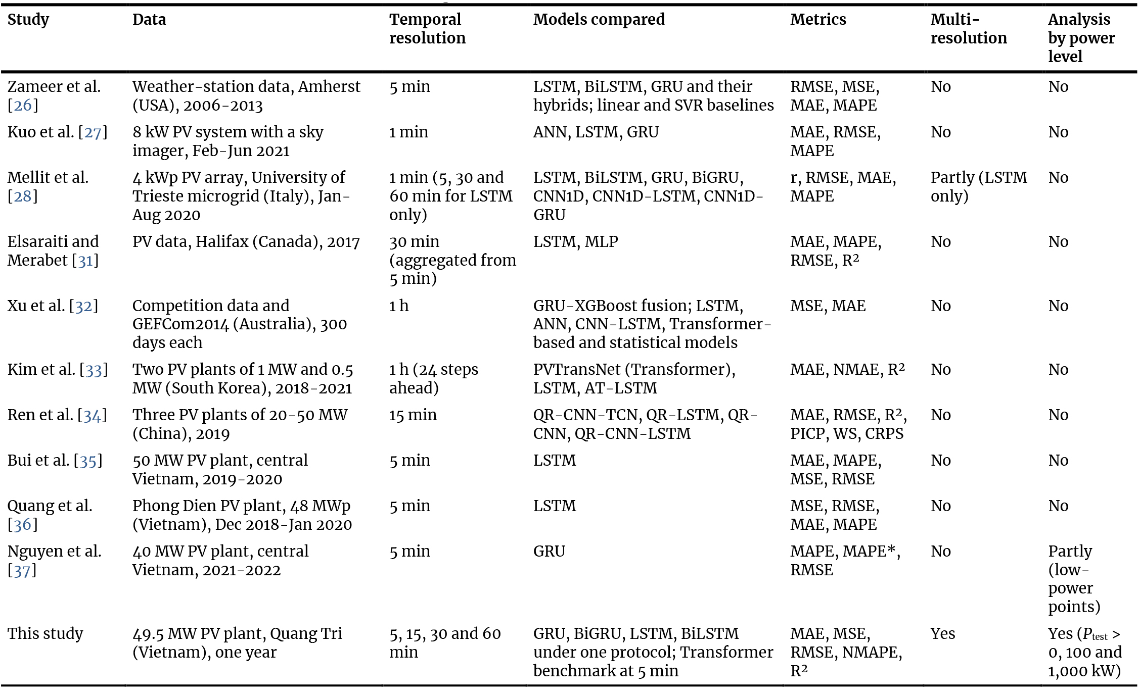
Table 1. Comparison of representative solar power forecasting studies with this study.
Globally, there have been numerous case studies employing RNN-based models to forecast solar power generation. These studies often utilize high-quality datasets from experimental PV installations and evaluate multiple deep learning configurations under different forecasting horizons. For instance, researchers in [28] trained LSTM, BiLSTM, GRU, and BiGRU models using power data from the University of Trieste microgrid, while others proposed combinations of GRU and gradient boosting (XGBoost) to improve long-term solar forecasting [32]. A comprehensive study explored the state of PV power forecasting and highlighted a growing trend in using advanced RNN models. It was found that case studies published in 2022 and 2023 commonly utilized LSTM, BiLSTM, GRU, and BiGRU models, underlining the increasing relevance of these architectures in this domain [38]. Despite this progress, the majority of existing works adopt heterogeneous datasets, preprocessing pipelines, and evaluation metrics, which limits the comparability and generalizability of their findings.
More recently, attention-based deep learning architectures have attracted considerable interest in PV power forecasting. Transformer models and their efficient variants, such as Informer [39], dispense with recurrence and rely on self-attention to capture long-range dependencies, and several recent studies have applied them to multi-step and ultra-short-term PV forecasting with encouraging results [33], [40]. In parallel, explainable artificial intelligence techniques have been coupled with solar forecasting models to interpret the contribution of individual meteorological drivers [41], while probabilistic formulations based on quantile regression provide uncertainty intervals in addition to deterministic point forecasts [34]. Nevertheless, Transformer-based models are generally data- and computation-intensive and tend to excel at longer horizons, whereas gated RNN variants remain highly competitive for single-plant, short-horizon applications with moderate data volumes. A systematic understanding of how these established RNN variants behave across temporal resolutions therefore remains a necessary reference baseline, both for practitioners and for future comparisons against attention-based and probabilistic approaches.
In Vietnam, several studies have also investigated the use of RNN-based models for solar power forecasting. However, the majority of these efforts have focused primarily on LSTM and GRU. For example, LSTM has been applied to forecast power generation of large-scale solar plants considering seasonal weather variability [35], [36], and a GRU model has been used for short-term load forecasting in the Vietnamese power system [42]. LSTM has also been applied to a solar plant operating under curtailment [43], while GRU has been utilized for forecasting using historical datasets from central Vietnam [37]. Additionally, there have been efforts to integrate LSTM or GRU with other models, such as ANN, to enhance prediction performance [44]. Despite these advancements, the studies in Vietnam tend to rely on unidirectional and standalone RNN models, with limited consideration of the superior predictive capacity of bidirectional configurations like BiGRU and BiLSTM. Existing research suggests that these bidirectional models generally outperform their unidirectional counterparts due to their ability to process input sequences in both forward and backward directions, thereby capturing more contextual information [45].
Another limitation observed in the literature is the lack of comparative studies evaluating the performance of different RNN-based models under a unified experimental framework. Given the heterogeneity among solar power plants, including differences in geographic location, weather patterns, and system configurations, it is crucial to conduct research that not only compares model performance but also develops tailored models specific to each power plant. Moreover, there is a need to establish a standardized methodology that guides the entire forecasting pipeline, from data acquisition and preprocessing to model training and performance evaluation. Such a framework would enable the identification of optimal models suited to the specific characteristics of each solar installation. Importantly, without a controlled experimental setup, it is difficult to isolate whether observed performance differences arise from model architecture or from external factors such as data quality and preprocessing choices.
An additional area that merits attention is the inconsistency in the use of performance metrics across different studies. While some research evaluates models using Mean Absolute Error (MAE), Root Mean Squared Error (RMSE), and Mean Absolute Percentage Error (MAPE) [26], [27], [29] or only RMSE and MAPE [30], others employ different combinations, including Mean Squared Error (MSE), coefficient of determination (R²), Symmetric Mean Absolute Percentage Error (SMAPE), and Mean Relative Error (MRE) [44], [46], [47], [48]. This inconsistency makes it difficult to directly compare results across studies. In contrast, some researchers argue that the use of a comprehensive set of metrics provides a more reliable and well-rounded evaluation of model performance [49]. Therefore, future research should aim to incorporate a broader suite of evaluation indicators to facilitate meaningful comparisons and benchmarking across studies.
Another important research gap lies in the evaluation of forecasting models across different temporal resolutions. Existing studies often focus on fixed forecasting intervals, such as 5, 30 or 60 minutes, without analyzing how model performance varies across these time scales. For instance, [50] evaluated solar energy prediction at 10-minute resolutions, while [48] assessed performance at 5-minute intervals. However, few studies have explicitly investigated which models are best suited for different temporal resolutions. More importantly, the fundamental reasons why forecasting difficulty changes across temporal resolutions, such as information loss due to aggregation, smoothing effects, and changes in temporal dependency structures, remain insufficiently explored. This is a critical issue, as forecasting needs differ depending on the application context. Short-term forecasts (e.g., minutes to one hour ahead) are essential for real-time control, energy pricing, and optimal operation scheduling. Mid-term forecasts (e.g., one day to several days ahead) are more suitable for generating unit control, maintenance planning, and risk management. Long-term forecasts (e.g., months to one year ahead) are primarily used for system planning and site selection of solar plants. Therefore, selecting models that align with the specific forecasting interval and application context is crucial. There is a need for comprehensive research that compares model performance across multiple temporal resolutions and identifies the optimal forecasting strategy for each use case.
Based on the above gaps, this study aims to address the key following research question:
- How does temporal resolution interact with the architectural characteristics of RNN-based models to influence forecasting performance in short-term solar power prediction?
- How does forecasting performance vary across different temporal resolutions and what underlying data characteristics contribute to these variations?
- How do different RNN architectures respond to changes in temporal resolution, and what explains the observed shift in model superiority across forecasting intervals?
- How do data-related factors, including input feature selection, outlier handling, and power distribution characteristics, influence model performance across different temporal resolutions?
- What practical insights can be derived regarding the selection of appropriate RNN architectures for different operational forecasting scenarios?
1.3. Research contribution
This study offers several novel contributions to the field of solar power forecasting, particularly in the context of deep learning-based time-series prediction. First, this research presents a comprehensive comparative analysis of advanced RNN-based models, including GRU, BiGRU, LSTM, and BiLSTM, some of which, particularly BiGRU and BiLSTM, have rarely been applied or evaluated in the context of solar power forecasting. By integrating bidirectional architectures, this study demonstrates their potential in capturing complex temporal dependencies in solar generation data. Unlike conventional benchmarking studies, all models are implemented under a unified and controlled experimental framework, ensuring that performance differences can be attributed primarily to architectural characteristics rather than external factors.
Second, it provides a systematic and comparative analysis of single-step photovoltaic (PV) power forecasting conducted across multiple temporal resolutions, including 5 minutes, 15 minutes, 30 minutes, and 60 minutes. The proposed framework adopts temporal aggregation to formulate forecasting as a single-step prediction problem at each time scale. This design enables a structured investigation of how temporal resolution affects forecasting difficulty and model behavior, rather than treating each resolution independently. This design could reduce forecasting complexity and enable efficient and consistent performance across multiple very short-term intervals, which are particularly relevant for real-time monitoring, operational control, and grid integration of solar power.
Third, the research introduces a structured evaluation framework using consistent and widely accepted performance metrics, including MAE, MSE, RMSE, NMAPE, and R². This not only ensures a fair comparison across models and forecasting intervals but also addresses inconsistencies found in prior works regarding evaluation standards. Furthermore, the analysis is extended to different output power thresholds, providing insights into model behavior under varying generation conditions, a factor that is rarely considered in prior research. In addition, the study provides empirical evidence that model superiority is not universal but depends on temporal resolution, offering practical guidance for selecting appropriate models in different operational scenarios.
Taken together, the fundamental novelty of this study lies not in proposing a new network architecture, but in the controlled empirical evidence that the three contributions above jointly provide: (i) a unified, single-site experimental design that isolates the effect of architectural characteristics (gating complexity and directionality) from confounding factors that hinder cross-study comparisons; (ii) the systematic documentation of a resolution-dependent crossover in model superiority - BiGRU dominates at the 5-30-minute resolutions while BiLSTM becomes superior at the one-hour resolution - which, to the best of the authors' knowledge, has not been explicitly quantified for a utility-scale PV plant in a tropical monsoon climate; and (iii) a mechanistic explanation linking this crossover to measurable data characteristics (autocorrelation decay, sample-size reduction, and the smoothing of cloud-induced ramps under temporal aggregation), which yields direct model-selection guidance for grid operators forecasting at different resolutions for different operational tasks.
To achieve the study’s contribution, the paper is organized as follows: Section 2 provides an overview of the study workflow and the forecasting models used; Section 3 describes the dataset and preprocessing steps; Section 4 presents empirical results; Section 5 discusses key insights and model performance; and Section 6 concludes with key findings and suggests future directions.
2. Methodology
2.1. Study workflow
This study proposes four advanced RNN variants, namely GRU, BiGRU, LSTM, and BiLSTM, for short-term PV power forecasting under dynamic environmental conditions. The overall workflow is shown in Figure 1. First, data from the selected PV plant, including environmental variables, generated power, and timestamps, are collected and pre-processed to extract relevant features. After normalization, the dataset is divided into training and testing sets. Outlier removal is applied only to the training data to improve model learning. The cleaned data are then used to train the proposed models, which are subsequently saved and evaluated on the testing set using standard performance metrics.
Figure 1
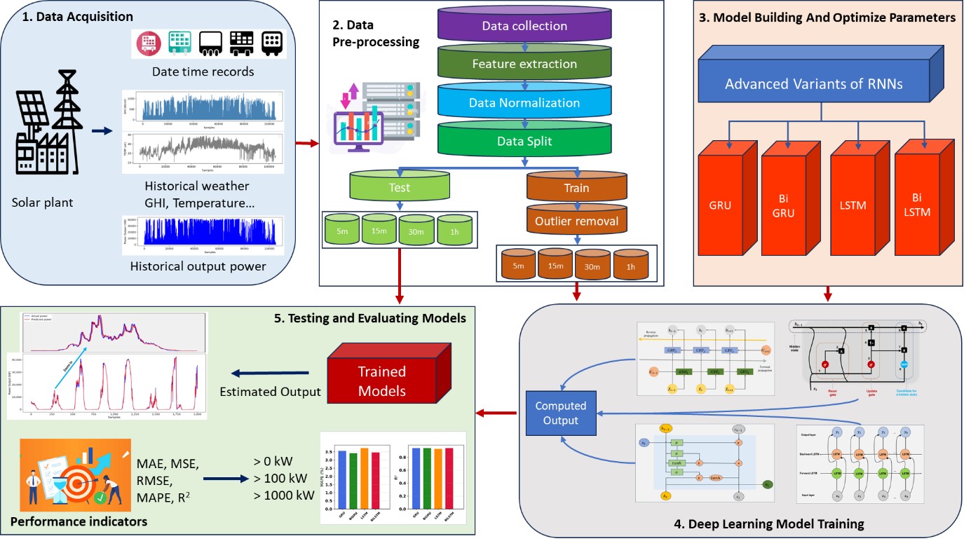
Fig. 1. Proposed workflow for advanced RNN-based forecasting models.
2.2. Time series deep learning models
2.2.1. Recurrent neural networks (RNNs)
RNNs are deep learning models designed to capture sequential dependencies through internal memory mechanisms. Unlike traditional neural networks that treat inputs independently, RNNs account for temporal order, making them suitable for sequential tasks [51]. By applying recurrent loops, RNNs generate outputs based on both current inputs and prior states [52]. This temporal awareness is advantageous in applications such as natural language processing, video analysis, and speech recognition, where context is essential [53], [54]. However, standard RNNs suffer from short-term memory limitations, hindering long-sequence learning [55]. To address this, advanced variants have been developed, including GRU [56], LSTM [57], bidirectional GRU [58], bidirectional LSTM [59]. Figure 2 illustrates the architecture of a basic RNN.
Figure 2
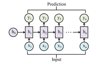
Fig. 2. Basic RNN architecture.
2.2.2. Gated recurrent unit (GRU)
GRU is a refined variant of the RNN designed to mitigate the limitations of short-term memory in conventional RNNs, while maintaining a more compact architecture than LSTM networks [51]. Introduced by Cho et al.[60], GRU simplifies the gating mechanism by merging the input and forget gates found in LSTM into a single update gate, thereby reducing computational complexity. The internal configuration of a GRU unit is illustrated in Figure 3 [61].
Figure 3
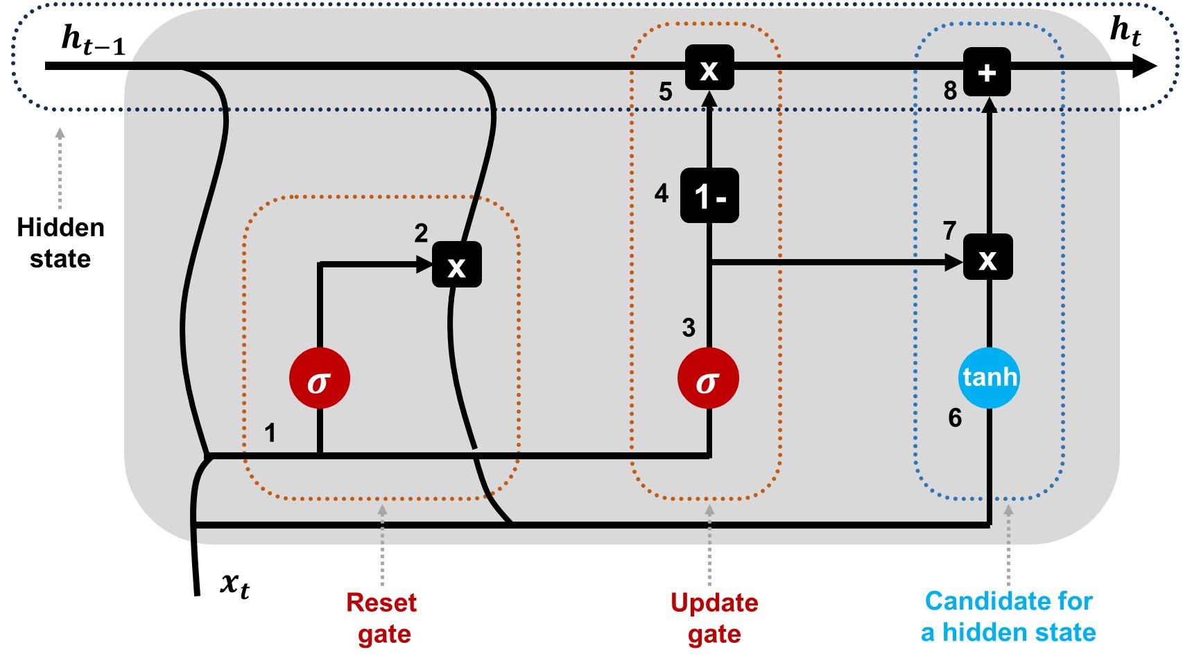
Fig. 3. Architecture of the GRU network.
Compared to LSTM, GRUs are computationally more efficient due to their simpler architecture, yet still capable of capturing long-term dependencies and mitigating the vanishing gradient problem. Their performance has been shown to be comparable to LSTM across various sequence modeling tasks [62], [63].
2.2.3. Bidirectional gated recurrent unit (BiGRU)
As an evolution of the GRU network, the BiGRU integrates bidirectional processing for improved sequence modeling [64]. In other words, BiGRU enhances the standard GRU model by incorporating information from both preceding and succeeding elements within a sequence [65]. Unlike the traditional GRU, which operates solely in a forward temporal direction, the BiGRU captures dependencies from both directions by employing two GRU layers simultaneously, one that reads the input sequence from start to end and another that reads it in reverse [66]. A diagram of the BiGRU model is illustrated in Figure 4.
Figure 4
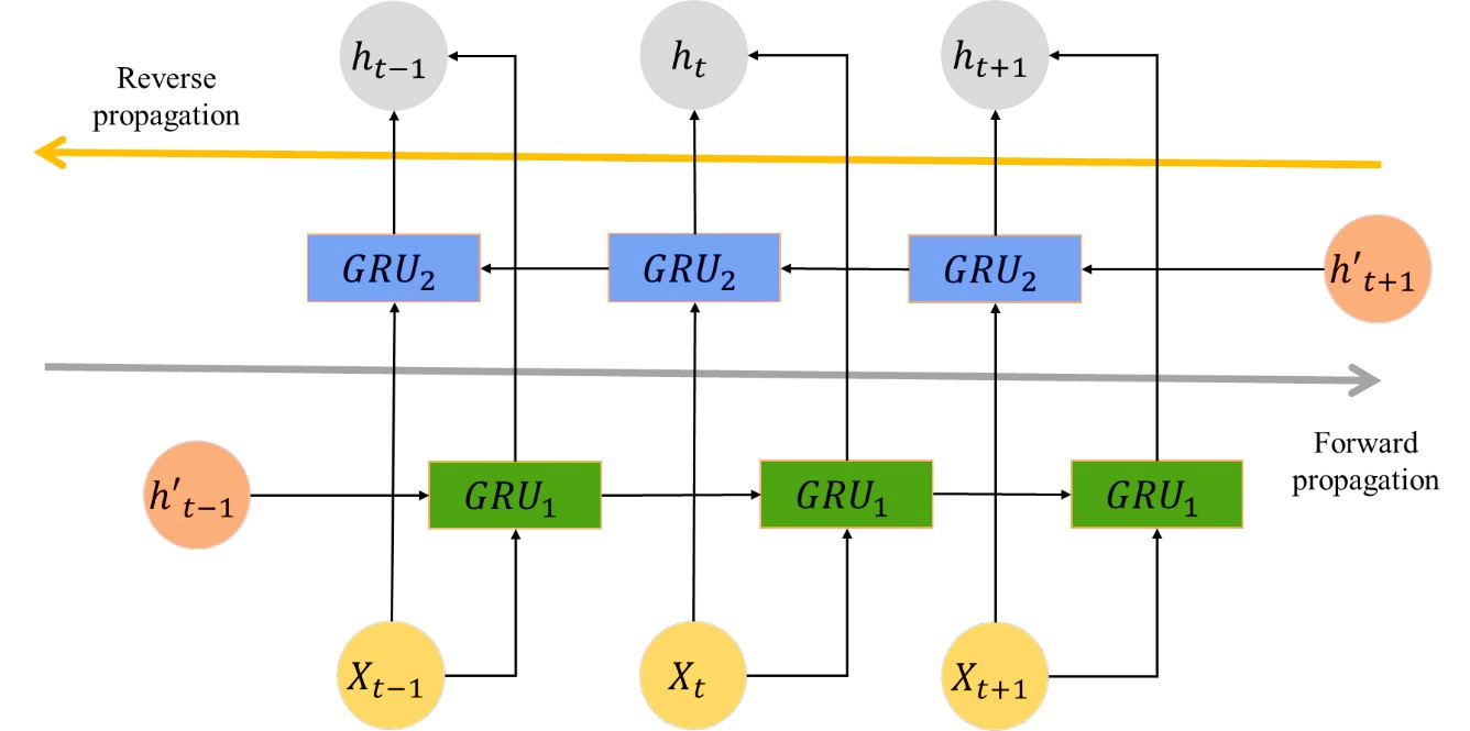
Fig. 4. Schematic diagram of the BiGRU model.
2.2.4. Long Short-Term Memory (LSTM)
LSTM is an advanced architecture within the RNN family, designed to address the challenge of learning long-term dependencies in sequential data. It was initially proposed in 1997 [57] and later improved with practical enhancements that increased its efficiency and stability [67] Compared to traditional RNNs, LSTM networks are more capable of preserving relevant information across extended sequences, which has led to their widespread adoption in deep learning applications [68], as shown in Figure 5 below.
Figure 5
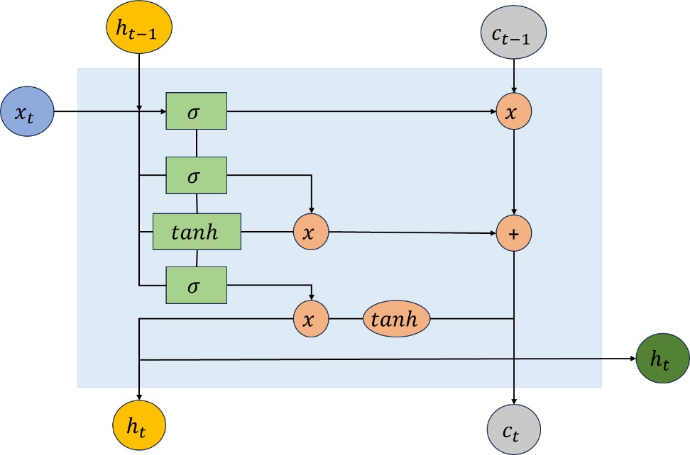
Fig. 5. Architecture of the LSTM network.
At each time step, an LSTM unit processes both the current input and the previous hidden state, producing an output that is passed on to the next time step. This mechanism enables the model to maintain a memory of prior events while updating it dynamically. The output of the final hidden layer, or in some applications, the collection of all hidden layers is commonly used for classification tasks [69].
2.2.5. Bidirectional long short-term memory (BiLSTM)
Bi-LSTM networks represent a significant advancement over traditional LSTM models, particularly in tasks that require a deeper understanding of sequential data. While standard LSTM architectures process information in a unidirectional manner, typically from past to future, Bi-LSTM enhances this by learning temporal dependencies in both directions [70]. The BiLSTM structure is shown in Figure 6 below.
The Bi-LSTM structure integrates two separate LSTM layers operating in parallel: one traverses the input sequence from left to right (forward direction), and the other processes it in the opposite direction, from right to left (backward direction) [71]. Through this bidirectional flow, the model gains access not only to historical context but also to future context within the input sequence.
Figure 6
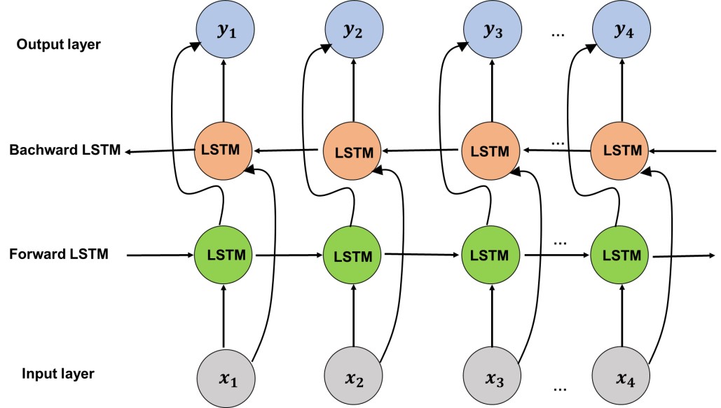
Fig. 6. Schematic diagram of the BiLSTM model.
2.3. Performance indicators
To evaluate forecasting performance, five metrics were used: MAE, MSE, RMSE, Normalized Mean Absolute Percentage Error (NMAPE), and R². These metrics are determined as Equations (1), (2), (3), (4), and (5), respectively. MAE measures the average absolute prediction error, while MSE and RMSE quantify squared and root-squared errors, giving greater weight to large deviations. NMAPE expresses the prediction error as a percentage of actual values and is commonly used in forecasting studies [48], [72]. However, because NMAPE is sensitive to very small or zero power values, zero-output samples were excluded and progressive filtering was applied to reduce distortion from low-power periods. R² was also used to assess the proportion of variance explained by the model, but it was interpreted together with error-based metrics because it does not directly reflect the absolute magnitude of forecasting errors.
In above equations, and denote the actual and forecasted values, respectively. The parameter represents the installed capacity of the photovoltaic (PV) system under study (in this case, = 49,500 kW, corresponding to a solar PV plant located in the central region of Vietnam), denotes the total number of data samples, and represents the mean of the actual (measured) values used in the R² denominator. All error metrics are computed on de-normalized (original-scale) data, and the same definitions apply at every temporal resolution.
2.4. Model configuration and hyperparameter settings
All four models were implemented in TensorFlow/Keras under an identical training protocol, so that performance differences can be attributed to architectural characteristics rather than tuning effort. The final configurations (Table 2) were selected through preliminary trial-and-error experiments, in which the number of recurrent layers, hidden units, and dropout rates were varied and the configuration with the most stable validation loss was retained; no automated hyperparameter optimization (e.g., grid or Bayesian search) was applied, which is acknowledged as a limitation and left for future work.
Table 2

Table 2. Architecture and hyperparameter settings of the four RNN-based models.
All models shared the same settings: a 12-step input window with a single-step-ahead target; Min-Max normalization of inputs and target to [0, 1], fitted on the training set only; the Adam optimizer (initial learning rate 0.001); the MSE loss; a batch size of 64; and a fixed training budget of approximately 4,600 gradient updates per run on the 5-minute dataset, within which the training and validation losses plateaued without overfitting. To account for stochastic initialization, each configuration was trained five times independently and the run with the lowest NMAPE was retained.
Computationally, all four models are lightweight by modern deep-learning standards: even the largest network (BiGRU) stores fewer than 2.4 x 10⁵ weights (below 1 MB in single precision), and a single forecast requires only a few million multiply-accumulate operations, far below the timing constraints of 5-minute operational forecasting. Because the training protocol was identical, relative training cost scales directly with the parameter counts in Table 2: the GRU cell requires roughly 25% fewer parameters than the LSTM cell owing to its two-gate structure, and bidirectional variants approximately double the cost of their unidirectional counterparts. Wall-clock times, by contrast, depend on the hardware and software environment and transfer poorly across platforms, so these hardware-independent indicators are reported instead. In this light, BiGRU is the most accurate model at a computational cost that remains trivial for operational deployment, while the unidirectional GRU offers the best accuracy per parameter where the computational budget is the binding constraint.
3. Data collection
3.1. Collecting data
The dataset consists of one year of 5-minute interval data collected from a 49.5 MW solar power plant in Quang Tri Province, Vietnam. The site is located in a climatic transition zone affected by tropical storms and the Foehn wind effect, leading to strong short-term variations in solar irradiance and temperature. The dataset includes solar radiation, ambient temperature, module surface temperature, time-related variables, and generated power. These variables allow the forecasting models to capture both meteorological variability and temperature-induced PV performance changes. An overview of the dataset is shown in Figure 7.
Figure 7
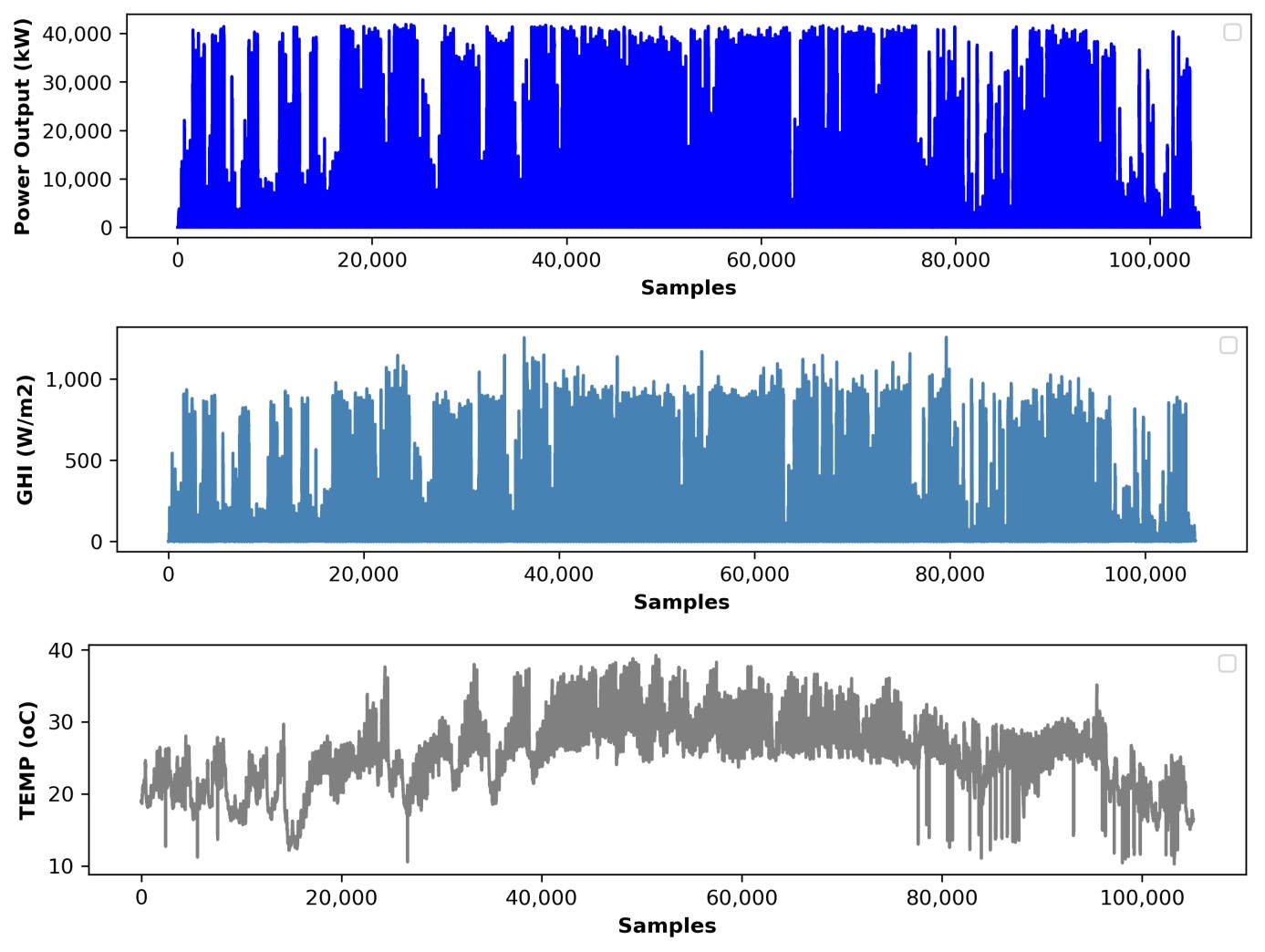
Fig. 7. Power output, GHI, and temperature of the plant during the observation period.
Figure 8 illustrates the variation in daily power output of the solar power plant throughout the month of April. As observed, the generated power fluctuates significantly from day to day throughout the month which can likely be attributed to changes in weather conditions. These fluctuations highlight the sensitivity of solar generation to meteorological factors.
Figure 8
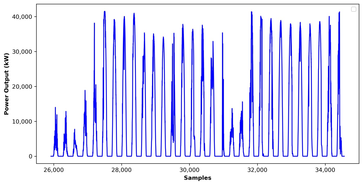
Fig. 8. Example of monthly power output in the dataset (April).
Figure 9 provides a typical daily power output profile, specifically for April 8. It is evident that the plant operates for approximately 11 to 12 hours per day, typically starting around 6 a.m. and ceasing generation by 5 p.m. This corresponds to the expected solar window during this time of year.
Figure 9
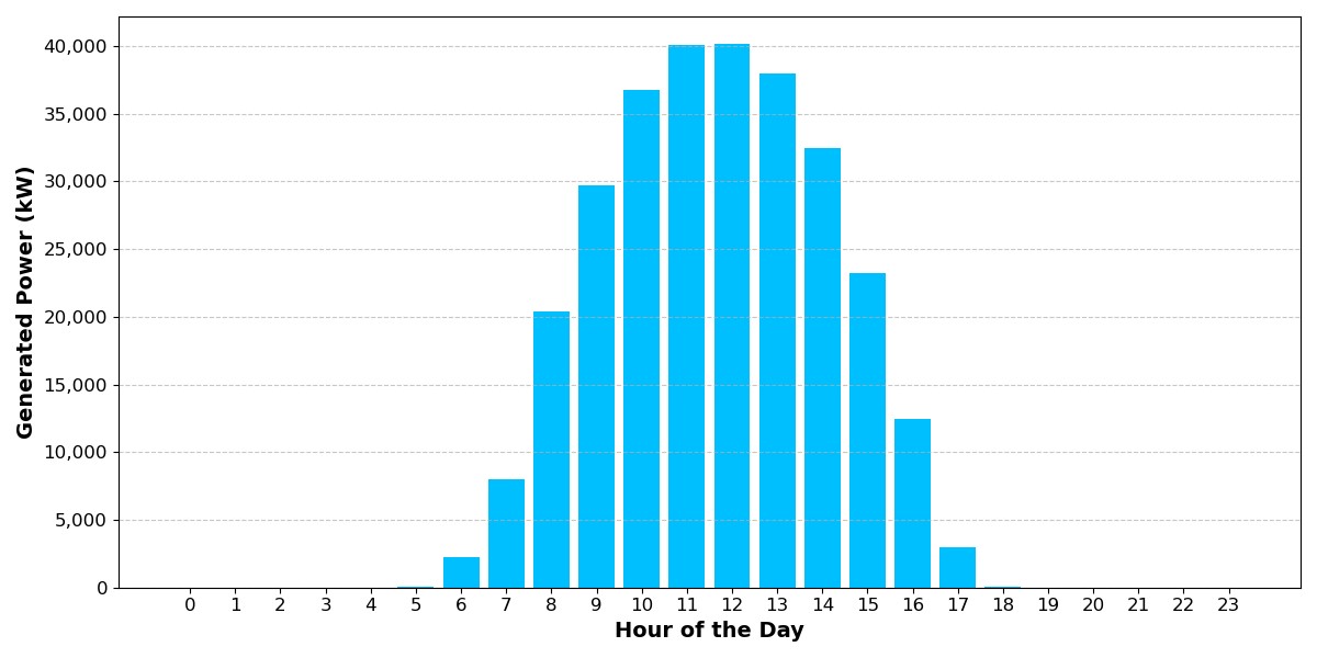
Fig. 9. Example of daily power output in the dataset (April 8).
The monthly characteristics of the dataset are summarized in Table 3, including generated power, average output, peak power, temperature, solar radiation, generation hours, and output variability.
Table 3 shows a clear seasonal pattern in solar power generation. The highest total generation occurred in June, reaching approximately 91.5 million kWh, followed by July and August, mainly due to higher solar radiation and longer generation hours. In contrast, December and February recorded the lowest generation levels, reflecting reduced irradiance and shorter daylight duration. Although monthly total and average generation varied substantially, peak power remained relatively stable at around 41 MW, indicating that the installed capacity was unchanged and that energy yield was mainly driven by seasonal and meteorological conditions.
Figure 10 further illustrates the monthly variation in total generated power, average output, and peak power. The figure confirms the strong increase in generation from March to September, with the highest output in June. The relatively stable peak power across months suggests consistent plant operation during optimal sunlight periods, while variations in total generation are mainly associated with changes in solar radiation and daylight hours.
Figure 10
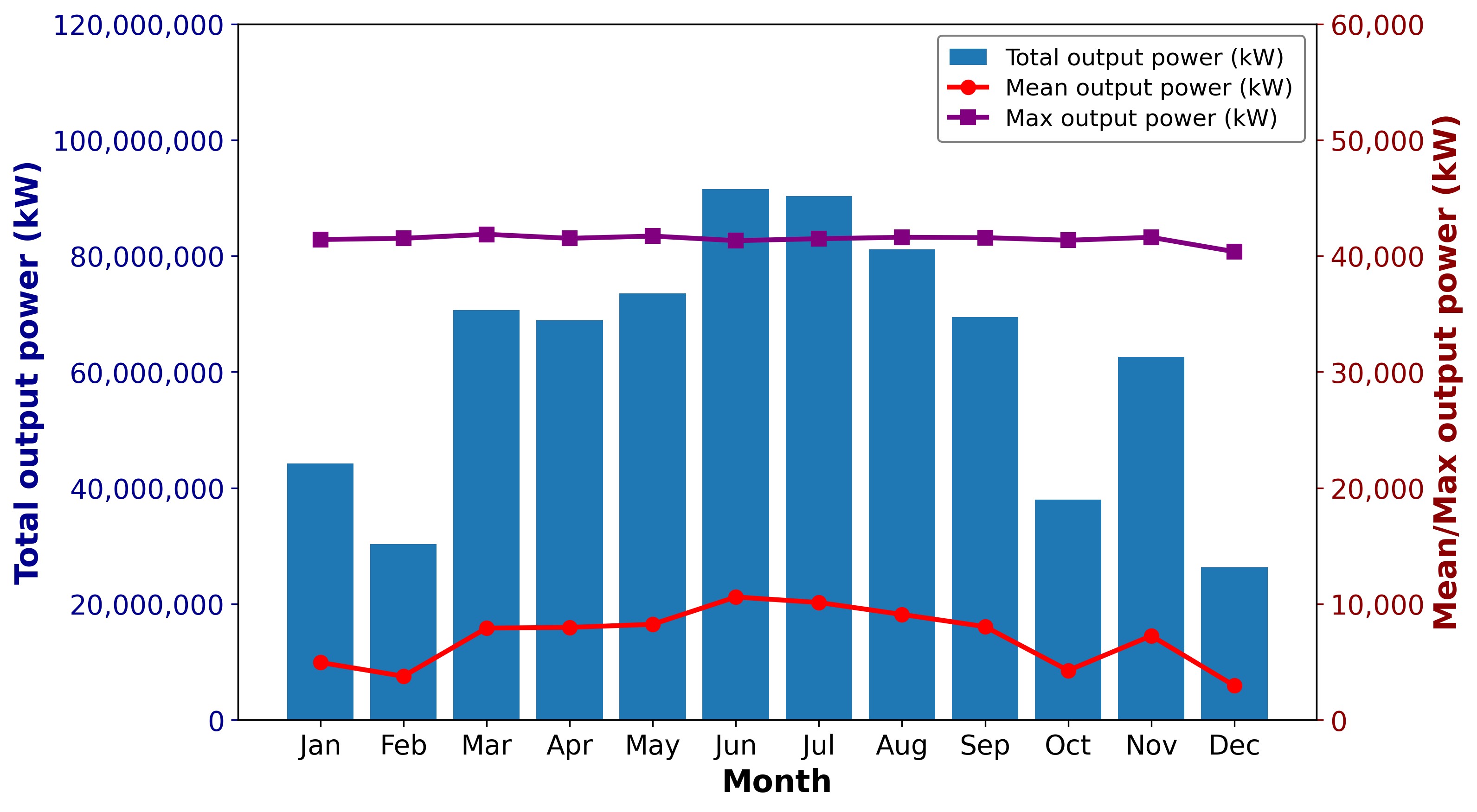
Fig. 10. Monthly solar power generation statistics.
Table 3
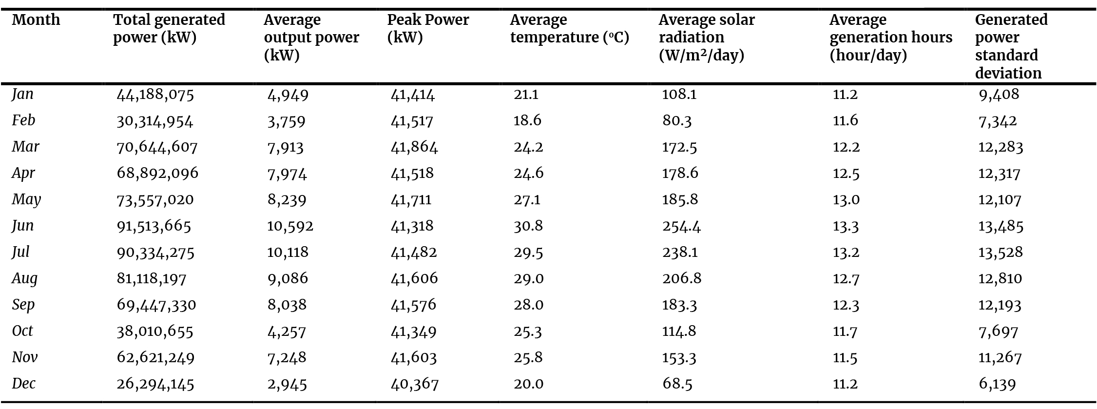
Table 3. Monthly summary of key solar power generation parameters at the solar power plant.
3.2. Data processing
From the raw dataset, key environmental and temporal features were prepared for solar power forecasting. The hour variable was converted into cyclic components (sin_hour and cos_hour), and a day_night feature was added to distinguish generation and non-generation periods.
The complete preprocessing pipeline can be summarized as follows. First, all sensor channels (power, irradiance, and temperatures) were aligned on a common 5-minute timestamp grid, and the coarser 15-, 30-, and 60-minute datasets were generated from this base series by averaging the records falling within each aggregation window, so that the aggregated series preserve the physical units and the diurnal envelope of the original data. Second, records containing missing or physically implausible sensor values were screened out during quality control, together with the radiation-power outlier filtering described below. Third, nighttime records were retained and explicitly flagged through the day_night variable so that the models learn the full diurnal cycle, whereas zero-power (non-generation) samples were excluded from the NMAPE-based evaluation, and results are additionally reported for progressively higher power thresholds (P > 0 kW, P > 100 kW, and P > 1,000 kW) to limit distortion from low-power periods. Fourth, anomalous records were removed from the training set only, while the test set was left untouched to reflect realistic operating conditions. Finally, all input features and the target variable were normalized to the range [0, 1] using Min-Max scaling fitted exclusively on the training data, and all forecasts were transformed back to physical units (kW) before any error metric was computed.
Figure 11 presents the correlation between the input features and power output. Solar radiation shows the strongest correlation with power generation (r = 0.987), followed by cell temperature (r = 0.893), day_night (r = 0.612), and ambient temperature (r = 0.560). In contrast, cos_hour shows a negative correlation (r = -0.699), reflecting the daily solar generation cycle. Feature selection was guided jointly by the Pearson correlation analysis and domain knowledge. Variables exhibiting a strong association with the power output (radiation, temperature_cell, temperature, and day_night) were retained, and the paired cyclic encodings sin_hour and cos_hour were kept together to preserve a unique, continuous representation of the time of day, while the calendar month was included to convey seasonal context. In addition, the historical generated power itself was included in the input vector, so that each model receives autoregressive information alongside the exogenous meteorological drivers. The resulting input vector therefore comprises eight features: radiation, temperature, temperature_cell, day_night, sin_hour, cos_hour, month, and the lagged generated power.
Figure 11
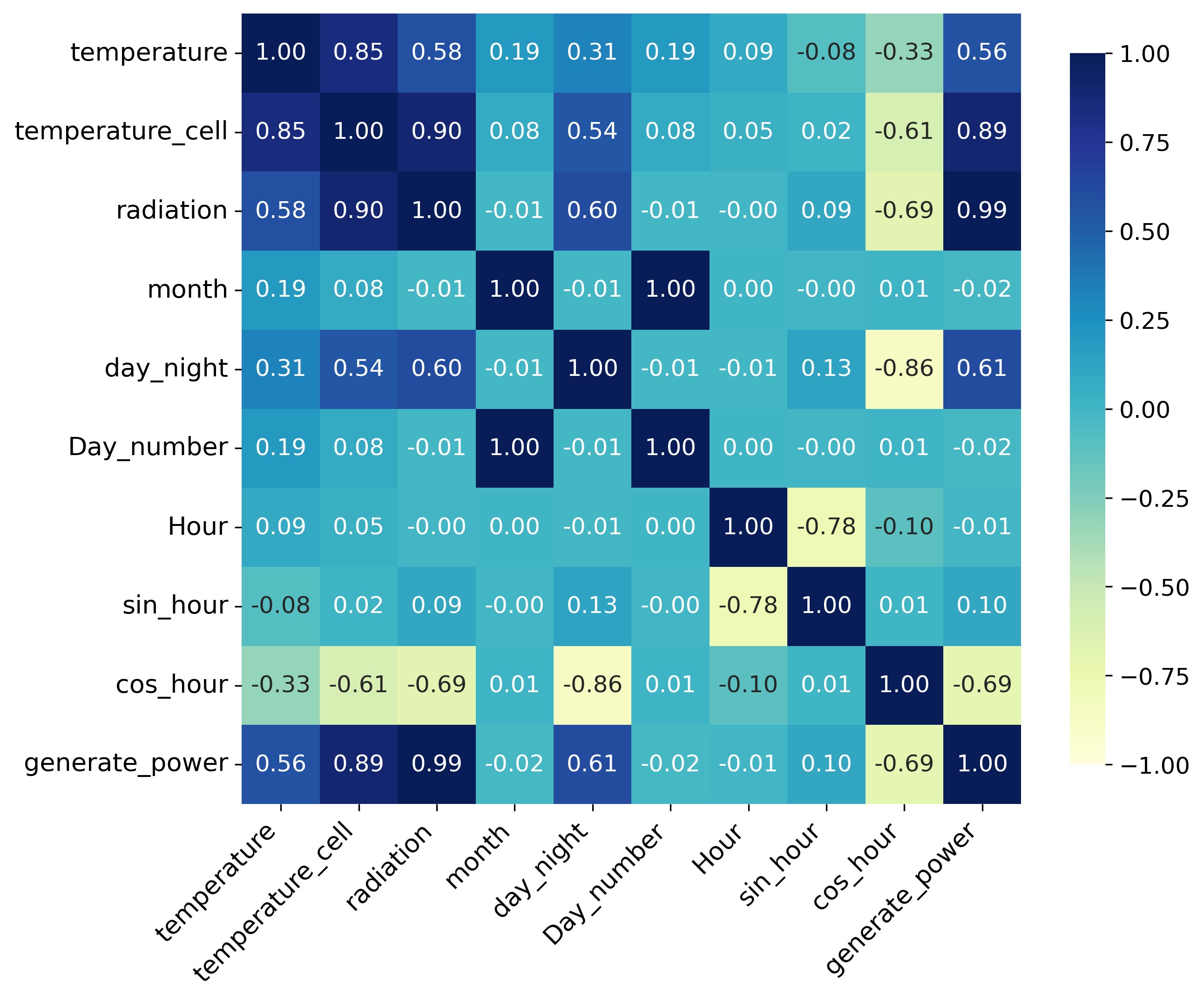
Fig. 11. Correlation between input features and power output.
To preserve seasonal representation, the 3rd, 6th, 13th, 16th, 23rd, and 26th days of each month were assigned to the test set, while the remaining data were used for training. This resulted in 19.7% testing data and 80.3% training data.
Outliers were removed from the training set using the radiation–power relationship and a 95% prediction interval. As shown in Figure 12, 3,790 anomalous records were excluded, leaving 97,540 data points for the 5-minute forecasting task.
Figure 12
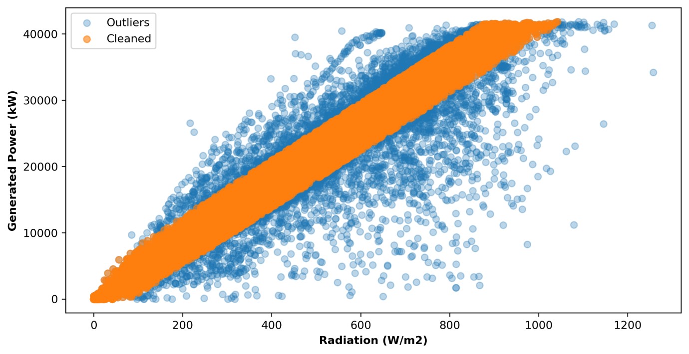
Fig. 12. Result of outlier removal based on the radiation–power relationship.
4. Results
This section summarizes the model results for different forecasting time resolutions. Additionally, the results are also aggregated across different power output ranges of the solar power plant, corresponding to electricity generation during various time periods throughout the day.
4.1. Forecasting results for the 5-minute interval
The performance of four deep learning models, including GRU, BiGRU, LSTM, and BiLSTM, was evaluated for 5-minute solar power forecasting across three power output scenarios: Ptest > 0 kW, Ptest > 100 kW, and Ptest > 1,000 kW. The results are summarized in Table 4 below:
Table 4
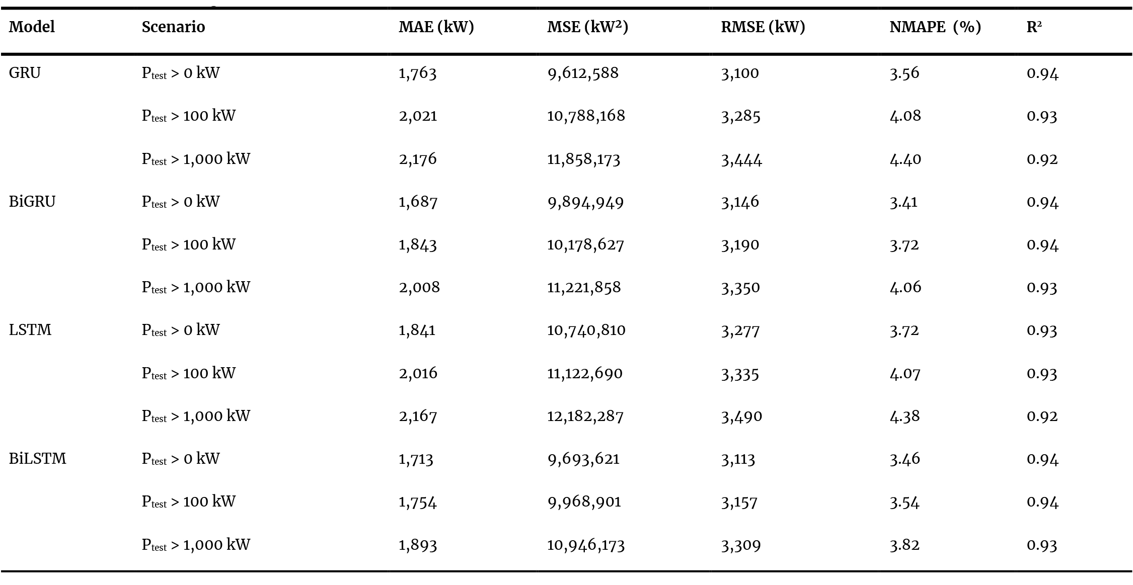
Table 4. 5-minute forecasting performance results.
Referring to Table 4 above, among the models, BiGRU consistently achieved the best performance, showing the lowest MAE, RMSE, and NMAPE values across all scenarios while maintaining high R² scores (~0.94). This indicates that BiGRU is highly effective for very short-term forecasting tasks. This trend is also clearly illustrated, as shown in Figure 13, which compares actual and predicted power values for the different models. From the graph, we can observe that all models perform relatively well, with predicted values closely aligning with actual measurements; however, BiGRU shows the highest degree of similarity, further confirming its high accuracy.
Figure 13
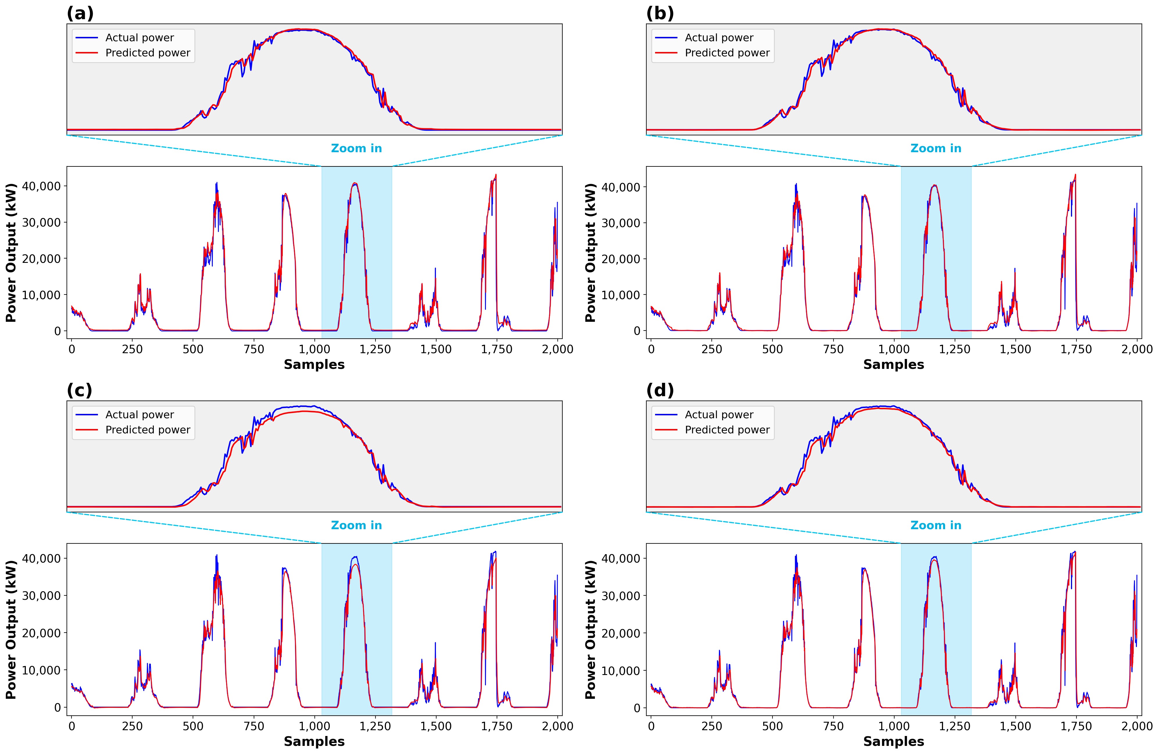
Fig. 13. 5-Minute interval forecasting — (a) BiGRU, (b) GRU, (c) LSTM, (d) BiLSTM.
For 5-minute forecasting resolution, GRU ranked second in performance, showing slightly higher error metrics than BiGRU but still yielding reliable accuracy. BiLSTM performed comparably to GRU in the lower and middle output ranges but slightly outperformed it at higher thresholds. LSTM, in contrast, produced the highest errors across all metrics, indicating its relative limitations in this context. As the power output threshold increased, all models exhibited higher errors, reflecting greater variability in power generation during peak sunlight hours. Nevertheless, BiGRU retained strong predictive accuracy, especially in the Ptest > 1,000 kW scenario, with the lowest RMSE (3,350 kW) and NMAPE (4.06%). Notably, the bidirectional models (BiGRU and BiLSTM) generally outperformed their unidirectional counterparts, highlighting the benefit of incorporating both past and future temporal contexts in short-term forecasting models.
Refer to Figure 14, examined models tend to perform better at lower power output levels. As the actual power increases, the predicted values tend to deviate downward from the reference line, indicating a consistent underprediction at higher power levels.
Figure 14
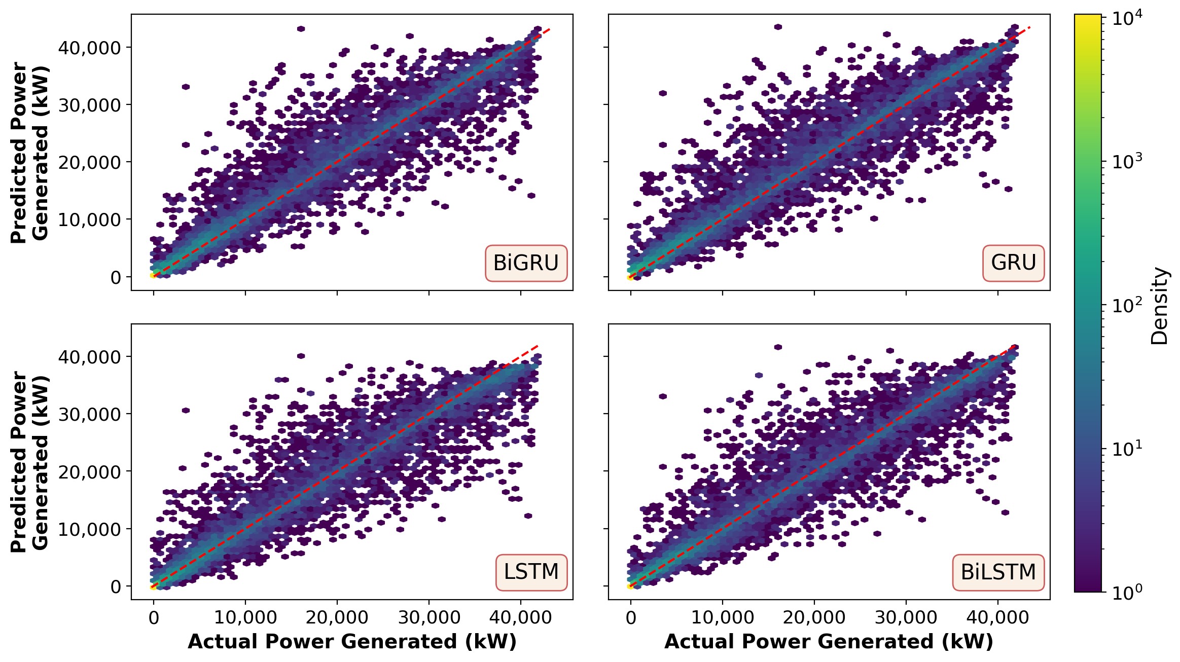
Fig. 14. Model accuracy evaluation via density plot (5-minute forecasting).
4.2. Forecasting results for the 15-minute interval
Table 5 below summarizes the forecasting performance of four deep learning models, including GRU, BiGRU, LSTM, and BiLSTM, over a 15-minute prediction interval.
Table 5
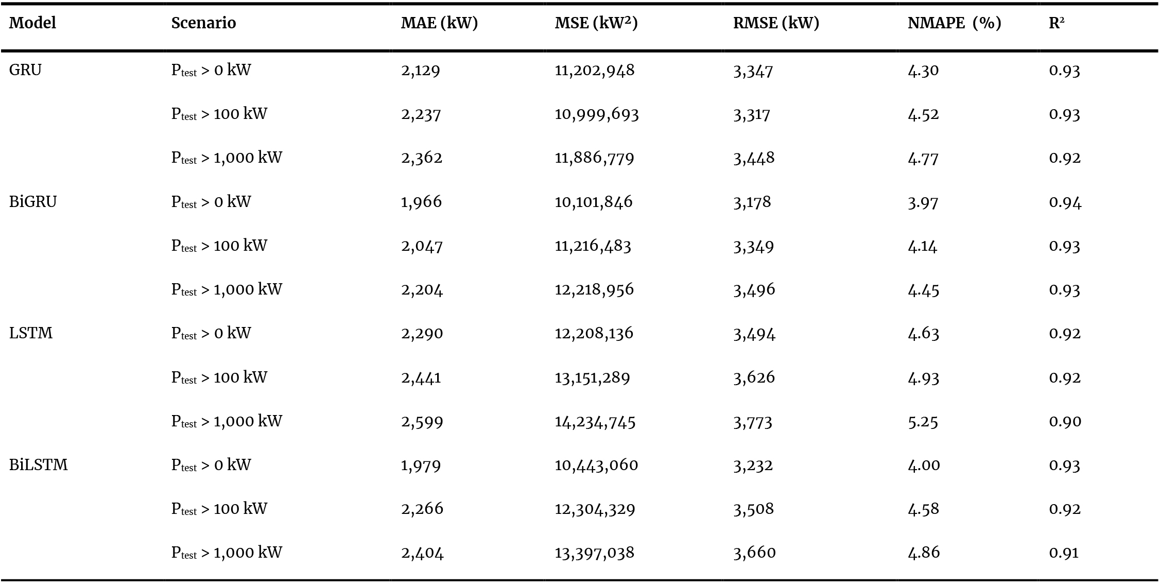
Table 5. 15-minute forecasting performance results.
For 15-minute resolution and under the full dataset scenario, the BiGRU model still demonstrates the best overall performance, achieving the lowest MAE (1,966 kW), RMSE (3,178 kW), and NMAPE (3.97%), while also maintaining a high R² score of 0.94. This indicates a strong fit between the predicted and actual values. BiLSTM followed closely with MAE and RMSE values of 1,979 kW and 3,232 kW, respectively, and an R² of 0.93. In contrast, the LSTM model showed the weakest performance in this scenario, with the highest MAE (2,290 kW), RMSE (3,494 kW), and the lowest R² (0.92), suggesting limitations in capturing short-term dependencies in the time series data.
As the minimum power output threshold increased, all models experienced a decline in performance. This trend is evidenced by rising MAE, RMSE, and NMAPE values, along with decreasing R² scores across all scenarios. For example, the GRU model's MAE increased from 2,129 kW to 2,362 kW and R² dropped from 0.93 to 0.92 as the threshold changed from Ptest > 0 kW to Ptest > 1,000 kW. This could suggest that forecasting becomes more challenging as the power output rises, likely due to increased variability and complexity in high-power scenarios.
Among the four models, BiGRU consistently delivered the most robust and stable performance across all power thresholds. Even under the high-power scenario (Ptest > 1,000 kW), BiGRU maintained relatively low errors (MAE = 2,204 kW, RMSE = 3,496 kW) and a strong R² value of 0.93. This implies that the bidirectional structure of BiGRU enhances its ability to capture both past and future context in sequential data, contributing to improved accuracy and generalization.
In contrast, the LSTM model continued to show relatively poor performance in high-power scenarios, with the highest observed MAE (2,599 kW) and the lowest R² (0.90), highlighting its limitations in effectively managing more complex patterns in the data. While BiLSTM showed improved results over LSTM, its performance still fell slightly behind BiGRU, particularly in scenarios involving higher power thresholds.
As seen in Table 5, the BiGRU model still emerged as the most suitable architecture for short-term solar power forecasting at a 15-minute resolution. Its superior accuracy and resilience across varying power levels make it a strong candidate for real-world applications where prediction reliability is critical. BiLSTM also provides a viable alternative with relatively strong results.
4.3. Forecasting results for the 30-minute interval
The forecasting performance of four proposed models was evaluated over a 30-minute interval, with the results outlined in Table 6.
Table 6
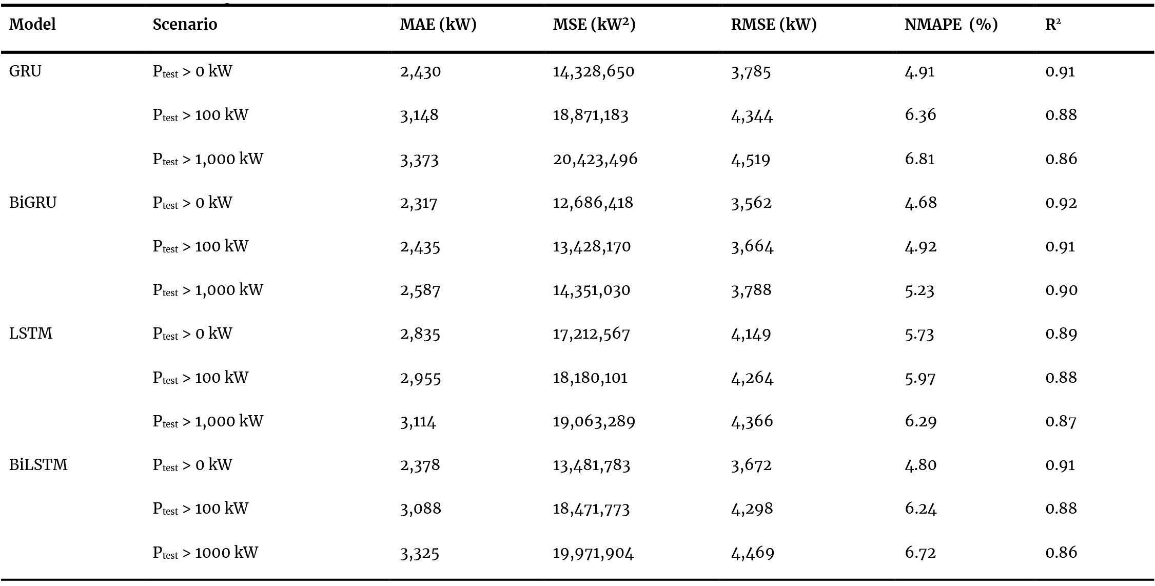
Table 6. 30-minute forecasting performance results.
As shown in the performance table, all models exhibit a general decline in accuracy compared to the 15-minute interval, which is expected due to the coarser temporal resolution. Among them, BiGRU consistently delivers the best overall performance, with the lowest MAE (2,317 kW), RMSE (3,562 kW), and NMAPE (4.68%) under the general scenario (Ptest > 0 kW), along with the highest R² value of 0.92. This suggests that BiGRU maintains robust predictive accuracy even over extended intervals.
GRU also performs relatively well, especially in lower-load scenarios, but shows a more noticeable drop in performance as the power level increases—its R² value falls from 0.91 to 0.86 when Ptest > 1,000 kW. Meanwhile, LSTM records the weakest performance across all metrics, particularly for higher power outputs, indicating its limitations in capturing longer temporal dependencies compared to gated recurrent variants. BiLSTM performs moderately, with accuracy falling between that of GRU and LSTM. However, it shows a substantial decline in performance under high-demand scenarios, with MAE rising to 3,325 kW and R² dropping to 0.86.
4.4. Forecasting results for the one-hour interval
The forecasting performance of four selected models over a one-hour prediction interval is gathered in Table 7 below.
Table 7
Table 7. One-hour forecasting performance results.
When extending the forecasting resolution to a one-hour interval, the predictive performance of the examined models further declines, reflecting the inherent difficulty of long-term solar power prediction due to insufficient historical data. Among the models, BiLSTM emerges as the most effective, particularly in low- and mid-range power scenarios, achieving the lowest RMSE (4,785 kW), MAE (3,471 kW), and NMAPE (7.01%) when Ptest > 0 kW, alongside an R² value of 0.85. These results suggest that BiLSTM can effectively retain and utilize longer-term sequential patterns, enhancing its stability over extended intervals.
While GRU continues to perform reasonably well in lower power output ranges, its prediction accuracy deteriorates significantly in high-power scenarios. Specifically, its R² value drops from 0.88 (Ptest > 0 kW) to 0.77 (Ptest > 1,000 kW), indicating increased error dispersion under more volatile conditions. BiGRU, although previously leading at shorter intervals, appears to struggle with one-hour forecasting, posting a higher MAE and RMSE than BiLSTM, especially for Ptest > 0 kW. However, its performance remains more consistent than LSTM’s.
LSTM demonstrates the weakest performance across all evaluated conditions, particularly at higher power levels. For instance, with Ptest > 1,000 kW, it yields the highest error values—MAE of 5,601 kW, RMSE of 7,140 kW, and NMAPE of 11.32%, with a relatively low R² of 0.64, signaling that its ability to generalize deteriorates significantly over extended time frames.
As observed from Figure 15, all four forecasting models perform well when actual power outputs vary smoothly. However, they face significant challenges in accurately predicting sudden fluctuations in power output.
Figure 15
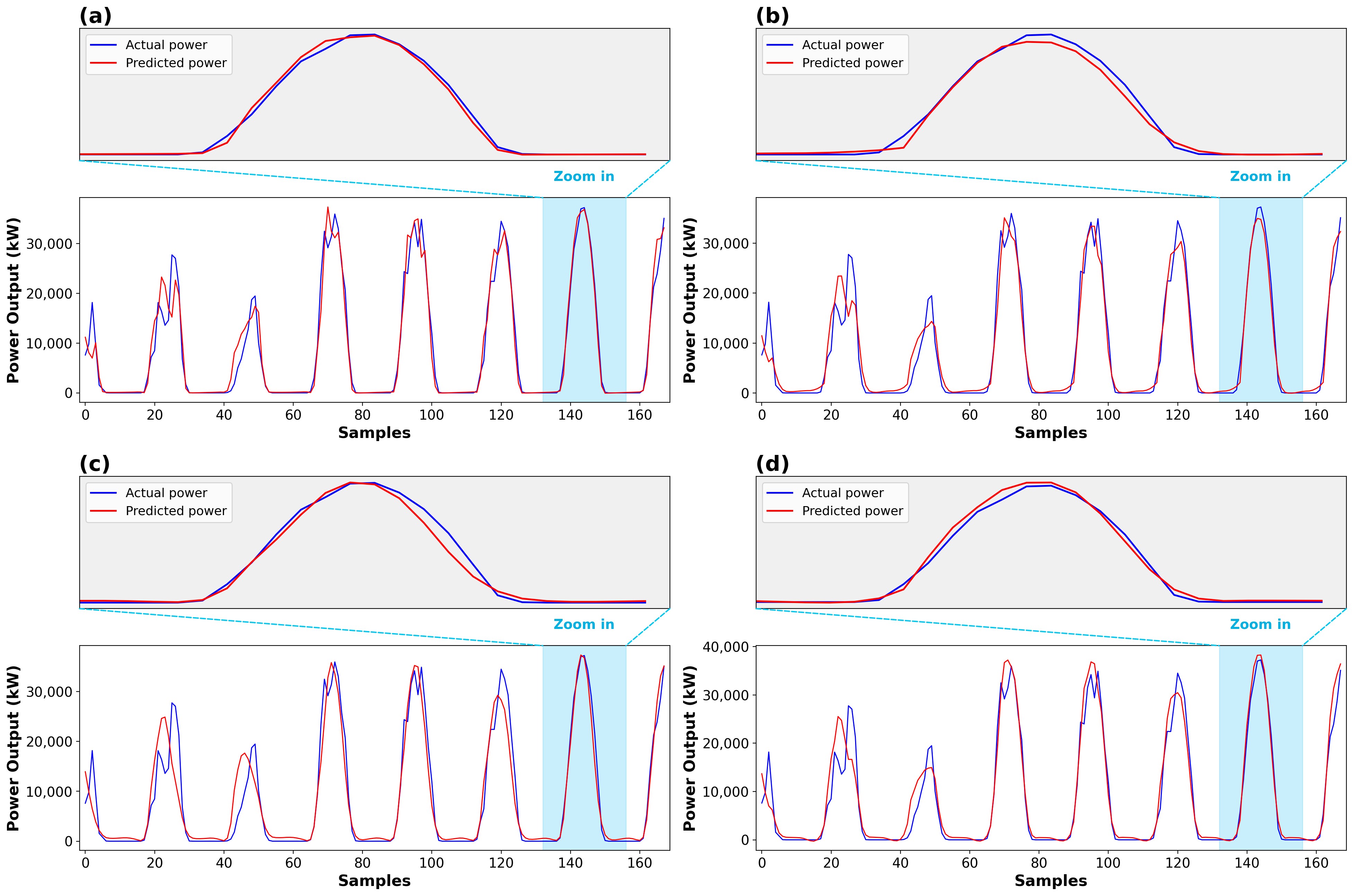
Fig. 15. One-hour interval forecasting — (a) BiGRU, (b) GRU, (c) LSTM, (d) BiLSTM.
Regarding Figure 16, although the number of data points significantly decreases in the one-hour forecasting interval, it is difficult to visually distinguish accuracy differences among the models based solely on the density plots. However, when combined with the summary in Table 7, it becomes evident that the prediction error widens noticeably over the one-hour interval, with LSTM exhibiting the highest variance. In contrast, BiLSTM demonstrates a tighter alignment with actual outputs, particularly in the mid-range power bands. These findings underscore BiLSTM’s relative advantage in long-term solar power forecasting while also highlighting the challenge of maintaining model accuracy as the forecast resolution extends.
Figure 16
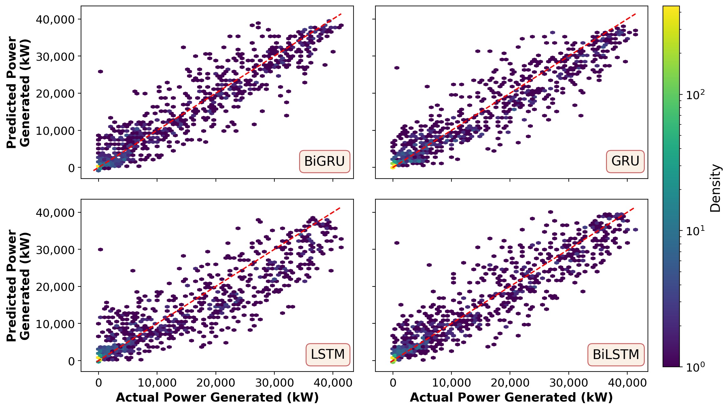
Fig. 16. Model accuracy evaluation via density plot (one-hour forecasting).
4.5. Benchmark comparison with a representative attention-based model
To situate the RNN family within the broader landscape of deep-learning forecasting approaches, an additional benchmark was conducted at the 5-minute resolution against a vanilla Transformer encoder, the archetypal member of the attention-based family emphasized in recent literature [33], [39], [40], whose popular variants (e.g., the Temporal Fusion Transformer) share the same core self-attention mechanism. The 5-minute resolution was chosen as the representative case because it is the headline operational resolution of this study and provides the largest training set, which is the most favorable condition for data-intensive attention models. The Transformer was evaluated under the identical experimental protocol used for the RNN models: the same eight input features, Min-Max scaling fitted on the training set only, a 12-step input window with a single-step target, the same optimizer, loss function, batch size, and epoch budget, and five independent training runs with the best run selected by NMAPE. The encoder uses a model dimension of 64, four attention heads, two encoder blocks, a feed-forward dimension of 128, a dropout rate of 0.1, and sinusoidal positional encoding, totaling 69,633 trainable parameters, which places it between the LSTM and BiLSTM in size. The results are summarized in Table 8, in which the best-performing RNN at this resolution (BiGRU) is reproduced from Table 4 for direct comparison.
Table 8
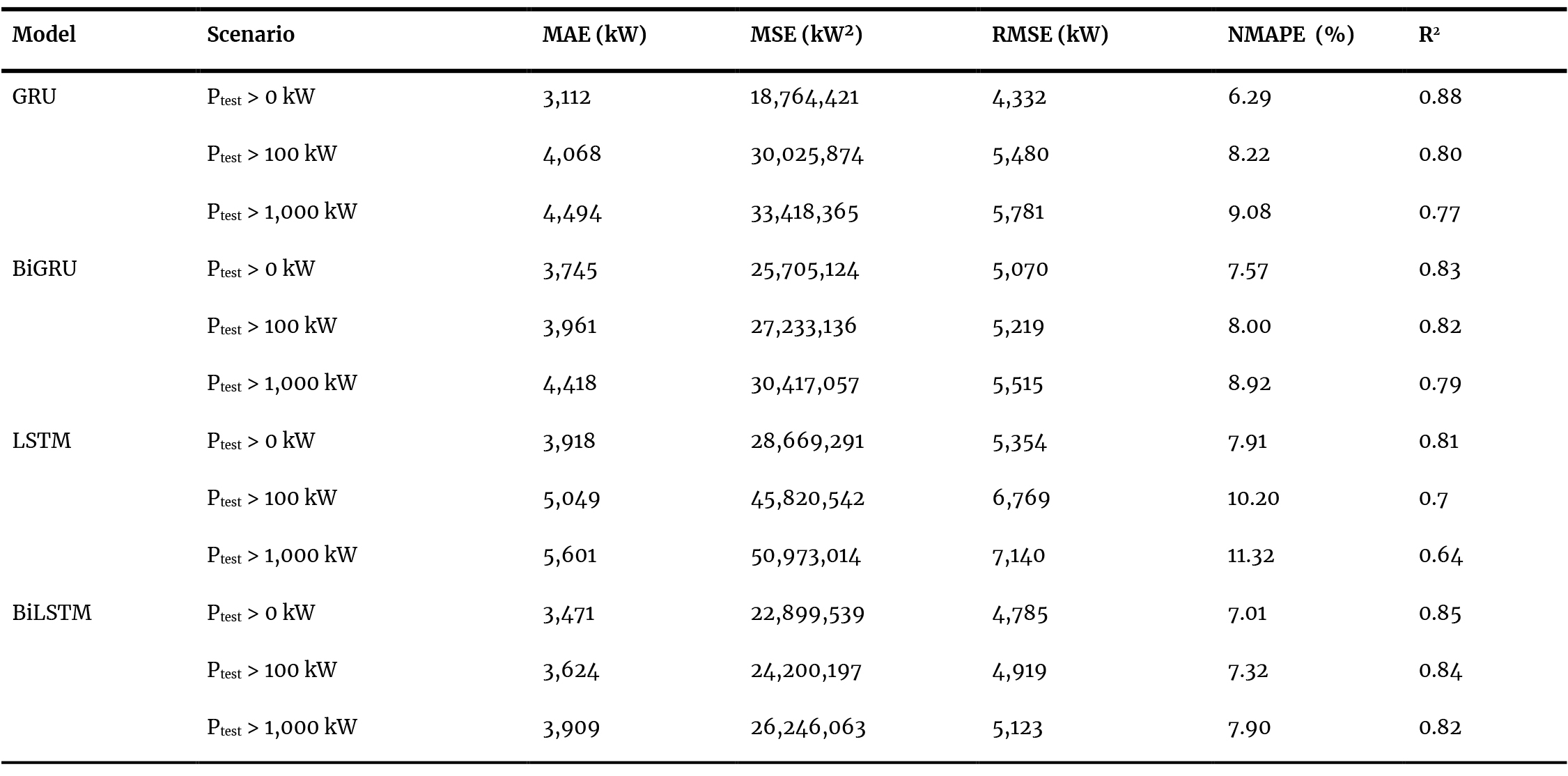
Table 8. Benchmark results of the vanilla Transformer at the 5-minute resolution, with BiGRU reproduced from Table 4 for comparison.
As shown in Table 8, the vanilla Transformer and the bidirectional RNNs occupy the same accuracy tier under the identical, deliberately modest training budget. BiGRU attains the lowest errors in the full-data scenario (NMAPE of 3.41% versus 3.54%, and MAE of 1,687 kW versus 1,754 kW), while the margins at the higher power thresholds are small in either direction, well within the modest-margin range discussed in Section 5.4. This parity indicates that, for single-plant, short-horizon forecasting with moderate data volumes, gated recurrent architectures remain fully competitive with attention-based models, which is consistent with recent comparative studies reporting that Transformers tend to show their clearest advantages at longer horizons and larger data scales [33], [39]. At the same time, attention architectures offer natural extensions toward multi-step decoding and probabilistic forecasting [34].
5. Discussion
5.1. Overall forecasting performance across forecast intervals
Figure 17 below illustrates the performance of the four proposed models in the task of solar power generation forecasting across four different forecast intervals within the scope of the study.
Figure 17
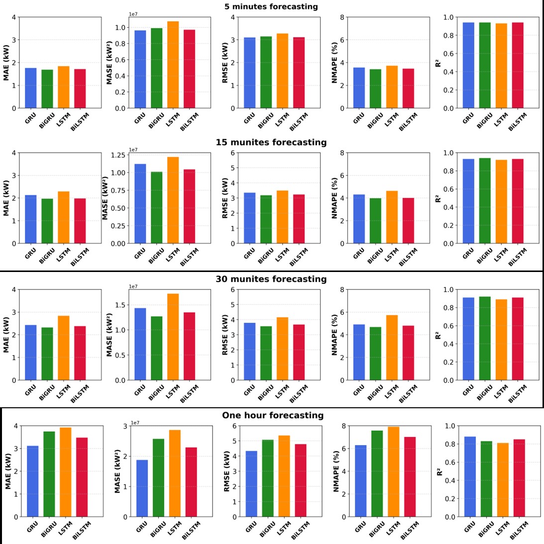
Fig. 17. Model performance across forecast intervals.
In relation to Figure 17, the forecasting performance tends to decline as the forecast interval increases. Specifically, at shorter intervals such as 5 and 15 minutes, the models achieve high accuracy with low MAE, RMSE, and NMAPE values, and high R² scores. However, performance significantly deteriorates at the 1-hour interval. This phenomenon can be explained by the fact that temporal aggregation reduces high-frequency variability while simultaneously introducing uncertainty due to information loss, making it more difficult for models to reconstruct short-term dynamics.
Among the compared models, BiGRU demonstrates superior performance across most time frames, particularly at the 5, 15, and 30-minute intervals. This highlights the advantage of the bidirectional architecture in capturing short-term temporal dependencies in the data. More specifically, the GRU structure, with its simpler gating mechanism compared to LSTM, is more responsive to rapid fluctuations in high-frequency data, allowing it to adapt quickly to short-term changes in solar irradiance. When combined with bidirectional learning, BiGRU effectively captures both immediate past and near-future context, which is particularly beneficial in short-interval forecasting where temporal continuity is strong. Conversely, LSTM tends to deliver the weakest results, with higher error metrics and lower R² values, especially at the 30-minute and 1-hour intervals. This may be attributed to its more complex gating structure, which can lead to slower adaptation to rapid changes and potential over-smoothing in highly dynamic conditions.
A more mechanistic explanation can be offered by considering how temporal aggregation alters the statistical structure of the series. Averaging twelve 5-minute records into an hourly value act as a low-pass filter: it attenuates the high-frequency, cloud-induced ramps that dominate sub-15-minute variability, but it also weakens the strong short-lag autocorrelation that short-horizon forecasters exploit. At fine resolutions, consecutive samples are highly correlated, so the forecasting problem is dominated by local pattern continuation; the compact two-gate GRU cell, with fewer parameters to fit (Table 2), adapts quickly to these local dynamics and is less prone to overfitting, while the backward pass of the bidirectional wrapper supplies additional context about the shape of the current ramp within the input window. As the resolution coarsens, each 12-step input window spans a progressively longer physical duration (one hour at the 5-minute scale versus half a day at the hourly scale), the number of training samples shrinks by a factor of twelve, and the residual predictable structure shifts from local continuation toward slower, weather-regime-scale dependencies. Under these conditions, the explicit cell state of the LSTM, with its separate input, forget, and output gates, becomes advantageous for retaining information across the longer effective horizon, which explains why BiLSTM overtakes BiGRU at the one-hour resolution. Physically, the plant's location in a climatic transition zone affected by tropical storms and the Foehn wind effect produces frequent abrupt irradiance transients; these transients are the dominant error source at fine resolutions, whereas at the hourly scale forecast errors are governed mainly by broader cloud-cover and weather-regime evolution.
5.2. Key input variables that significantly affect model performance
One of the key factors affecting the performance of solar power forecasting models is the distribution characteristics of the input power data. The experimental results in this study clearly demonstrate that deep learning models, particularly RNN architectures such as GRU, BiGRU, LSTM, and BiLSTM, tend to deliver more accurate forecasts at lower power levels, where fluctuations are less abrupt. This indicates that model performance is closely linked to the degree of nonlinearity and volatility present in the data, which varies not only with power levels but also across temporal resolutions. Conversely, as power levels increase, especially near peak capacity, the forecasting error also increases significantly. This is evident through the underestimation of predicted points relative to the reference line in the density plots. Such underestimation can be explained by the difficulty of capturing sudden irradiance drops (e.g., due to cloud movement), which become more pronounced when data is aggregated over longer intervals. These findings are consistent with other studies in literature. For example, a study by Nguyen Tuan Anh et al. using a GRU model showed that the NMAPE increased from 3.144% (for power values > 0 kW) to 3.52% (for power values > 1,000 kW) [37]. Another study at a power plant in central Vietnam reported a full-day NMAPE error (all-hour average) ranging from about 4.0% to 4.7%, while the NMAPE error from 6:00 to 18:00 rose to about 8.0% to 9.4% [35].
Outlier removal in the training dataset is also critical, as it significantly contributes to the quality of forecasting models. In this study, outliers were removed using the linear relationship between solar radiation and generated power. This preprocessing step ensures that the models learn the true physical relationship rather than noise, which is particularly important when comparing architectures under different temporal resolutions. This highlights the importance of selecting and processing input features, such as indicators related to solar irradiance, temperature, and on-site weather conditions. In a study using the LSTM model [73], the authors proposed replacing time-based variables with solar irradiance data under clear-sky conditions, which led to a significant performance gain, reducing NMAPE from 3.491% to 3.08%, an improvement of up to 12%. This helps reduce noise in model training. Moreover, developing additional features that are closely correlated with power generation, such as day/night classification or solar generation phase angles, could further enhance forecasting quality. These improvements suggest that feature engineering can partially compensate for information loss at coarser temporal resolutions.
Another important consideration is the method used to divide the training and test datasets. The test data should be evenly distributed across different time intervals instead of being concentrated at the end of the dataset. This helps avoid model bias and ensures that the model learns general trends and periodic patterns in both input and output variables. This is especially important when analyzing model behavior across temporal resolutions, as uneven sampling could distort the observed relationship between resolution and performance.
5.3. Developing and optimizing advanced RNN-based forecasting architectures
In this study, the performance of four deep learning models based on RNN architectures was thoroughly evaluated across different forecast intervals. Unlike conventional studies that focus only on accuracy, this analysis aims to explain how architectural differences influence learning behavior under varying temporal conditions. BiGRU consistently outperformed other models in short-term forecasts, particularly at the 5- and 15-minute intervals, achieving average R² values between 0.93–0.94 and NMAPE from 3.41% to 3.97%, respectively. This highlights the clear advantage of bidirectional models in leveraging both past and future context to improve accuracy. At short temporal resolutions, the strong autocorrelation in the data allows BiGRU to efficiently exploit local temporal patterns using its relatively lightweight gating mechanism.
GRU and BiLSTM models also performed well, while LSTM generally showed the weakest performance, especially in scenarios with high power output or coarser forecast intervals. Interestingly, at the 1-hour interval, BiLSTM outperforms BiGRU, which can be explained by its more complex memory cell structure. The input, forget, and output gates in LSTM allow it to retain long-term dependencies more effectively, which becomes critical when short-term information is lost due to temporal aggregation. In this context, the bidirectional nature of BiLSTM further enhances its ability to reconstruct broader temporal patterns, making it more suitable for coarser resolutions. This is aligned with the study that BiLSTM and BiGRU demonstrated superior predictive accuracy compared to their unidirectional counterparts [45].
Compared to previous studies conducted in the literature, the performance metrics in this study show promising potential for applying advanced variants of RNNs to solar power generation forecasting. In another study applying models such as CatBoost, LightGBM, and XGBoost, the R² value reached a maximum of only about 0.608 in the training set and 0.46 in the test set [74], which is significantly lower than the results achieved by BiGRU in this study. A separate study using the LSTM model [48], applied to the Thanh Cong 1 solar power plant, used forecasted weather data as input. The use of this data caused a significantly higher NMAPE compared to using historical weather data (10.857% versus 3.491%). However, after improving the model by incorporating new features and addressing forecast-related errors, the NMAPE was reduced to 9.881%. This indicates that even when changing the input data source (i.e., forecasted weather), the predictive model’s NMAPE remained relatively high. This further suggests that model architecture alone cannot guarantee performance; its effectiveness depends on how well it aligns with the temporal characteristics of the data.
5.4. Evaluating forecasting performance using multiple metrics
The simultaneous use of multiple evaluation metrics such as MAE, MSE, RMSE, NMAPE, MASE, and R² allows for a comprehensive assessment of model performance. In particular, R² evaluates how well the model fits the actual data, while NMAPE and MAE reflect the absolute and relative errors of the forecasts. In this study, BiGRU demonstrated stability by maintaining NMAPE at low values among other proposed models which is below 4.7% and R² above 0.92 in most scenarios (except one-hour forecasting interval), even under high power output conditions. This stability reflects its ability to generalize well under high-frequency conditions where local temporal dependencies dominate.
It is worth noting that, at the finest resolution, the margins separating the leading models are modest (e.g., an NMAPE of 3.41% for BiGRU versus 3.46% for BiLSTM at 5 minutes). The conclusions of this study are therefore not drawn from any single pairwise difference, but from the consistency of the observed ranking: BiGRU attains the lowest errors across all three power thresholds and at all three sub-hourly resolutions, while the reversal in favor of BiLSTM at the one-hour resolution is comparatively large (NMAPE of 7.01% versus 7.57%, and RMSE of 4,785 kW versus 5,070 kW). Moreover, every metric is computed over a large and chronologically representative test set (72 days evenly distributed across all twelve months of the year), and each architecture was trained five times under an identical protocol with the best run retained for every model, so that no architecture benefits from a more favorable training draw. Because the present work adopts a deterministic (point-forecast) formulation for a single plant, in which forecast errors of consecutive test samples are strongly autocorrelated, formal significance procedures designed for comparisons across many independent datasets, as well as probabilistic uncertainty intervals, fall outside its scope; extending the framework toward probabilistic forecasting, in which prediction intervals can be quantified explicitly [34], is identified as a direction for future work.
Compared to other studies [48], when LSTM was applied under different forecasted weather data conditions, where four performance metrics were employed, RMSE increased significantly from 996 kW to 3,216 kW, and NMAPE rose from 1.085% to 4.432%. Another study, which evaluated performance using only two metrics, NMAPE and RMSE, employed a white-box and combination model on two real-world datasets from Central Australia and Vietnam. The model achieved NMAPE and RMSE values of around 4% for real-time or intraday PV power prediction [50]. These comparisons highlight that a multi-metric evaluation framework is necessary to fully capture model behavior, especially when performance varies across temporal resolutions.
5.5. Forecasting performance across multiple temporal resolutions and model scalability
The ability of forecasting models to scale to coarser prediction intervals (such as one hour and one day) is a crucial requirement for practical applications, such as system planning, maintenance schedule [5], and it lays the foundation for the development of medium- and long-term prediction models. Based on the one-year dataset used in this study, the results show that while the BiGRU model outperforms others at shorter intervals, the BiLSTM model stands out at the 1-hour forecast window, achieving an MAE of 3,471 kW and a NMAPE of 7.01%. This transition in model superiority provides direct empirical evidence for the research question, confirming that temporal resolution and model architecture interact in a non-trivial way to determine forecasting performance. This indicates the flexibility in selecting models depending on operational requirements. However, all models exhibit a decline in performance as the forecast interval increases, especially under conditions of high-power output and significant fluctuations. This decline can be attributed to the combined effects of information loss, increased uncertainty, and reduced temporal resolution of key features. This presents a direction for future research to investigate the subjective and objective causes of these power output sudden fluctuations throughout the day, and to develop models capable of accurately predicting such volatile periods.
Moreover, it is important to emphasize that the number of published scientific studies on solar power forecasting in Vietnam remains limited. Most current solutions originate from commercial software, which does not publicly share source code or data [74], [75], creating challenges for system expansion and upgrades. Therefore, developing and comparing advanced predictive models in academic research is essential. On one hand, this helps evaluate the practical applicability of research models; on the other, it enables identification of strengths and weaknesses among models of the same family across multiple temporal resolutions, thereby paving the way for future work such as the development of hybrid models. More importantly, this study contributes to a deeper understanding of the mechanisms behind model performance variation, rather than merely reporting comparative results.
6. Conclusion
The growing penetration of solar photovoltaic energy presents significant challenges for grid operators, particularly in ensuring reliable, real-time power forecasting. This study evaluates and compares the performance of four advanced RNN architectures including GRU, BiGRU, LSTM, and BiLSTM, for short-term solar power forecasting at multiple temporally aggregated time resolutions: 5, 15, 30, and 60 minutes. Results demonstrate that all models perform reasonably well for short-term predictions, with BiGRU consistently outperforming the others across most forecasting intervals from 5 to 30 minutes. BiGRU achieved an R² of approximately 0.94 and a NMAPE as low as 3.41% at the 5-minute interval.
While BiGRU maintained strong performance up to 30 minutes (NMAPE = 4.68%, R² = 0.92), its accuracy declined at the 60-minute resolution (R² = 0.83). In contrast, BiLSTM demonstrated better performance at this coarser resolution, achieving R² = 0.85 and NMAPE = 7.01%, indicating its ability to capture long-range temporal dependencies. The analysis also revealed that forecasting accuracy tended to deteriorate as power output increased, particularly near peak output or during periods of rapid fluctuation. In addition, a benchmark against a representative attention-based baseline at the 5-minute resolution showed that a vanilla Transformer performs on par with the bidirectional RNNs under the same training budget, with BiGRU retaining the lowest overall errors, which confirms that gated recurrent architectures remain competitive with attention-based models for short-horizon, single-plant solar power forecasting.
Despite these promising results, the study is limited by its reliance on data from a single location, which may affect the generalizability of results. Additionally, while the temporal resolution aggregation employed in this study improves forecasting complexity and reduces high-frequency noise, it may limit the ability of the forecasting models to represent short-lived power ramps within each aggregated interval. Moreover, model accuracy declined at peak output levels and over longer time intervals, indicating difficulty in capturing extreme variations. Future work should incorporate multi-location datasets to improve robustness and explore hybrid models, such as BiGRU with Transformers or reinforcement learning, to better handle volatility. Enhancing input preprocessing and integrating real-time or external meteorological data may also help reduce forecast errors.
Funding
This research received no external funding.
Author Contributions
Ngoc-Trung Nguyen: Writing – original draft, Visualization, Software, Investigation. Thanh-Trung Nguyen: Writing – review & editing, Methodology, Formal analysis. Manh-Hai Pham: Writing – review & editing, Validation, Resources, Data curation. Nguyen Tuan Anh: Writing – review & editing, Validation, Data curation. Minh-Phap Vu: Writing – review & editing, Validation, Supervision, Methodology, Conceptualization.
Declaration of competing interest
The authors declares no conflicts of interest.
Declaration of generative AI and AI-assisted technologies
During the preparation of this work, the authors used ChatGPT and Claude in order to check spelling and improve the quality of the writing. After using this tool, the authors reviewed and edited the content as needed and take full responsibility for the content of the published article.
References
- M. A. Elhadidy, S. M. Shaahid, Parametric study of hybrid (wind + solar + diesel) power generating systems, Renewable Energy, 21:2 (2000) 129-139. https://doi.org/10.1016/S0960-1481(00)00040-9
- K. Wang, X. Qi, H. Liu, A comparison of day-ahead photovoltaic power forecasting models based on deep learning neural network, Applied Energy, 251 (2019) 113315. https://doi.org/10.1016/j.apenergy.2019.113315
- K. Wang, X. Qi, H. Liu, A comparison of day-ahead photovoltaic power forecasting models based on deep learning neural network, Applied Energy, 251 (2019) 113315. https://doi.org/10.1007/s42107-024-01249-9
- I. Citaristi, International energy agency-iea, in: The Europa directory of international organizations 2022, Routledge, 2022, pp. 701-702. https://doi.org/10.4324/9781003292548-126
- R. Asghar, F. R. Fulginei, M. Quercio, A. Mahrouch, Artificial Neural Networks for Photovoltaic Power Forecasting: A Review of Five Promising Models, IEEE Access, 12 (2024) 90461-90485. https://doi.org/10.1109/ACCESS.2024.3420693
- N. T. P. Thanh, Vietnam's Solar Energy Market: A Comprehensive Outlook for Investors, 2024. https://www.vietnam-briefing.com/news/vietnams-solar-energy-market-a-comprehensive-outlook-for-investors.html/
- M. Ha-Duong, Vietnam's Power Development Plan 8 (PDP8): A bold step towards a net-zero future, The Mekong Eye, 2023.
- C. Philibert, Solar energy perspectives, (No Title), 2011.
- H. Wang, Y. Liu, B. Zhou, C. Li, G. Cao, N. Voropai, E. Barakhtenko, Taxonomy research of artificial intelligence for deterministic solar power forecasting, Energy Conversion and Management, 214 (2020) 112909. https://doi.org/10.1016/j.enconman.2020.112909
- R. Ahmed, V. Sreeram, Y. Mishra, M. Arif, A review and evaluation of the state-of-the-art in PV solar power forecasting: Techniques and optimization, Renewable and sustainable energy reviews, 124 (2020) 109792. https://doi.org/10.1016/j.rser.2020.109792
- https://doi.org/10.1016/j.rser.2020.109792 https://doi.org/10.1016/j.solener.2014.10.016
- B. Uzum, A. Onen, H. M. Hasanien, S. M. Muyeen, Rooftop Solar PV Penetration Impacts on Distribution Network and Further Growth Factors-A Comprehensive Review, Electronics, 10:1 (2021) 55. https://doi.org/10.3390/electronics10010055
- B. Kraas, M. Schroedter-Homscheidt, R. Madlener, Economic merits of a state-of-the-art concentrating solar power forecasting system for participation in the Spanish electricity market, Solar Energy, 93 (2013) 244-255. https://doi.org/10.1016/j.solener.2013.04.012
- J. Antonanzas, N. Osorio, R. Escobar, R. Urraca, F. J. Martinez-de-Pison, F. Antonanzas-Torres, Review of photovoltaic power forecasting, Solar Energy, 136 (2016) 78-111. https://doi.org/10.1016/j.solener.2016.06.069
- B. Chen, P. Lin, Y. Lai, S. Cheng, Z. Chen, L. Wu, Very-short-term power prediction for PV power plants using a simple and effective RCC-LSTM model based on short term multivariate historical datasets, Electronics, 9:2 (2020) 289. https://doi.org/10.3390/electronics9020289
- T. Huld, G. Friesen, A. Skoczek, R. P. Kenny, T. Sample, M. Field, E. D. Dunlop, A power-rating model for crystalline silicon PV modules, Solar Energy Materials and Solar Cells, 95:12 (2011) 3359-3369. https://doi.org/10.1016/j.solmat.2011.07.026
- L. Visser, T. AlSkaif, W. van Sark, Operational day-ahead solar power forecasting for aggregated PV systems with a varying spatial distribution, Renewable Energy, 183 (2022) 267-282. https://doi.org/10.1016/j.renene.2021.10.102
- Z. Zhen et al., Deep learning based surface irradiance mapping model for solar PV power forecasting using sky image, IEEE Transactions on Industry Applications, 56:4 (2020) 3385-3396. https://doi.org/10.1109/TIA.2020.2984617
- A. Nespoli, E. Ogliari, S. Leva, A. Massi Pavan, A. Mellit, V. Lughi, A. Dolara, Day-ahead photovoltaic forecasting: A comparison of the most effective techniques, Energies, 12:9 (2019) 1621. https://doi.org/10.3390/en12091621
- S. Dutta et al., Load and renewable energy forecasting for a microgrid using persistence technique, Energy Procedia, 143 (2017) 617-622. https://doi.org/10.1016/j.egypro.2017.12.736
- A. Agga, A. Abbou, M. Labbadi, Y. El Houm, Short-term self consumption PV plant power production forecasts based on hybrid CNN-LSTM, ConvLSTM models, Renewable Energy, 177 (2021) 101-112. https://doi.org/10.1016/j.renene.2021.05.095
- N. D. Tuyen, N. T. Thanh, V. X. S. Huu, G. Fujita, A combination of novel hybrid deep learning model and quantile regression for short‐term deterministic and probabilistic PV maximum power forecasting, IET Renewable Power Generation, 17:4 (2023) 794-813. https://doi.org/10.1049/rpg2.12634
- M. O. Moreira, P. P. Balestrassi, A. P. Paiva, P. F. Ribeiro, B. D. Bonatto, Design of experiments using artificial neural network ensemble for photovoltaic generation forecasting, Renewable and Sustainable Energy Reviews, 135 (2021) 110450. https://doi.org/10.1016/j.rser.2020.110450
- S. Aslam, H. Herodotou, S. M. Mohsin, N. Javaid, N. Ashraf, S. Aslam, A survey on deep learning methods for power load and renewable energy forecasting in smart microgrids, Renewable and Sustainable Energy Reviews, 144 (2021) 110992. https://doi.org/10.1016/j.rser.2021.110992
- N. Bacanin, L. Jovanovic, M. Zivkovic, V. Kandasamy, M. Antonijevic, M. Deveci, I. Strumberger, Multivariate energy forecasting via metaheuristic tuned long-short term memory and gated recurrent unit neural networks, Information Sciences, 642 (2023) 119122. https://doi.org/10.1016/j.ins.2023.119122
- A. Zameer, F. Jaffar, F. Shahid, M. Muneeb, R. Khan, R. Nasir, Short-term solar energy forecasting: Integrated computational intelligence of LSTMs and GRU, Plos one, 18:10 (2023) e0285410. https://doi.org/10.1371/journal.pone.0285410
- W.-C. Kuo, C.-H. Chen, S.-Y. Chen, C.-C. Wang, Deep learning neural networks for short-term PV Power Forecasting via Sky Image method, Energies, 15:13 (2022) 4779. https://doi.org/10.3390/en15134779
- A. Mellit, A. M. Pavan, V. Lughi, Deep learning neural networks for short-term photovoltaic power forecasting, Renewable Energy, 172 (2021) 276-288. https://doi.org/10.1016/j.renene.2021.02.166
- S. khan, T. Mazhar, T. Shahzad, W. Waheed, A. Waheed, M. M. Saeed, H. Hamam, Optimizing deep neural network architectures for renewable energy forecasting, Discover Sustainability, 5:1 (2024) 394. https://doi.org/10.1007/s43621-024-00615-6
- [30] V. Gundu, S. P. Simon, Short term solar power and temperature forecast using recurrent neural networks, Neural processing letters, 53:6 (2021) 4407-4418. https://doi.org/10.1007/s11063-021-10606-7
- M. Elsaraiti, A. Merabet, Solar power forecasting using deep learning techniques, IEEE access, 10 (2022) 31692-31698. https://doi.org/10.1109/ACCESS.2022.3160484
- Y. Xu, S. Zheng, Q. Zhu, K.-c. Wong, X. Wang, Q. Lin, A complementary fused method using GRU and XGBoost models for long-term solar energy hourly forecasting, Expert Systems with Applications, 254 (2024) 124286. https://doi.org/10.1016/j.eswa.2024.124286
- J. Kim, J. Obregon, H. Park, J.-Y. Jung, Multi-step photovoltaic power forecasting using transformer and recurrent neural networks, Renewable and Sustainable Energy Reviews, 200 (2024) 114479. https://doi.org/10.1016/j.rser.2024.114479
- X. Ren, Y. Liu, F. Zhang, L. Li, A deep learning quantile regression photovoltaic power-forecasting method under a priori knowledge injection, Energies, 17:16 (2024) 4026. https://doi.org/10.3390/en17164026
- D. Bui, Q. Nguyen, V. Doan, T. Pham, D. Le, Evaluating an Effectiveness of a Solar Power Plant Output Forecasting Model Based on LSTM Method Using Validation in Different Seasons of a Year in Vietnam, GMSARN International Journal, 18:1 (2024) 114.
- N. Quang, L. Duy, B. Van, Q. Dinh, Applying Artificial Intelligence in Forecasting the Output of Industrial Solar Power Plant in Vietnam, EAI Endorsed Transactions on Energy Web (2021) 169166.
- T.-A. Nguyen, M.-H. Pham, V. M. Phap, Q.-H. Do, N.-T. Nguyen, D.-T. Nguyen, T. N. Nguyen, Forecasting of solar power generation in Vietnam deploying a simple GRU model, in: Proceedings of the 2023 Asia Meeting on Environment and Electrical Engineering (EEE-AM), IEEE, 2023, pp. 1-6. https://doi.org/10.1109/EEE-AM58328.2023.10395560
- S. Husein, E. Gago, B. Hasan, M. Pegalajar, Towards energy efficiency: A comprehensive review of deep learning-based photovoltaic power forecasting strategies, Heliyon, 2024. https://doi.org/10.1016/j.heliyon.2024.e33419
- H. Zhou, S. Zhang, J. Peng, S. Zhang, J. Li, H. Xiong, W. Zhang, Informer: Beyond efficient transformer for long sequence time-series forecasting, in: Proceedings of the AAAI Conference on Artificial Intelligence, 35:12 (2021) 11106-11115. https://doi.org/10.1609/aaai.v35i12.17325
- J. Wang, W. Hu, L. Xuan, F. He, C. Zhong, G. Guo, TransPVP: A transformer-based method for ultra-short-term photovoltaic power forecasting, Energies, 17:17 (2024) 4426. https://doi.org/10.3390/en17174426
- R. M. Rizk-Allah, L. M. Abouelmagd, A. Darwish, V. Snasel, A. E. Hassanien, Explainable AI and optimized solar power generation forecasting model based on environmental conditions, PLOS ONE, 19:10 (2024) e0308002. https://doi.org/10.1371/journal.pone.0308002
- T. H. B. Huy, D. N. Vo, H. D. Nguyen, H. P. Truong, K. T. Dang, K. H. Truong, Short-term load forecasting in power system using recurrent neural network, in: Proceedings of the 2023 International Conference on System Science and Engineering (ICSSE), IEEE, 2023, pp. 67-71. https://doi.org/10.1109/ICSSE58758.2023.10227203
- L. D. Bui, N. Nguyen Quang, E. R. Sanseverino, B. Doan Van, Forecasting Energy Output Solar Power Plant in Curtailment Condition Based on Lstm Using P/Ghi Factor and Validation in Training Process, a Case Study in Vietnam.
- T. A. Nguyen, M. H. Pham, T. K. Duong, M. P. Vu, A Recent Invasion Wave Of Deep Learning In Solar Power Forecasting Techniques Using Ann, in: Proceedings of the 2021 IEEE International Future Energy Electronics Conference (IFEEC), 16-19 November 2021, pp. 1-6. https://doi.org/10.1109/IFEEC53238.2021.9661747
- M. Jaihuni et al., A novel recurrent neural network approach in forecasting short term solar irradiance, ISA Transactions, 121 (2022) 63-74. https://doi.org/10.1016/j.isatra.2021.03.043
- A.-N. Buturache, S. Stancu, Solar energy production forecast using standard recurrent neural networks, long short-term memory, and gated recurrent unit, Engineering Economics, 32:4 (2021) 313-324. https://doi.org/10.5755/j01.ee.32.4.28459
- Y. Zhou, J. Wang, Z. Li, H. Lu, Short-term photovoltaic power forecasting based on signal decomposition and machine learning optimization, Energy Conversion and Management, 267 (2022) 115944. https://doi.org/10.1016/j.enconman.2022.115944
- N. Q. Nguyen, L. D. Bui, B. V. Doan, E. R. Sanseverino, D. D. Cara, Q. D. Nguyen, A new method for forecasting energy output of a large-scale solar power plant based on long short-term memory networks a case study in Vietnam, Electric Power Systems Research, 199 (2021) 107427. https://doi.org/10.1016/j.epsr.2021.107427
- R. C. Deo, M. Şahin, J. F. Adamowski, J. Mi, Universally deployable extreme learning machines integrated with remotely sensed MODIS satellite predictors over Australia to forecast global solar radiation: A new approach, Renewable and Sustainable Energy Reviews, 104 (2019) 235-261. https://doi.org/10.1016/j.rser.2019.01.009
- T. Nguyen‐Duc, H. Vu‐Xuan‐Son, H. Do‐Dinh, N. Nguyen‐Vu‐Nhat, G. Fujita, S. Tran‐Thanh, An adaptive method for real‐time photovoltaic power forecasting utilizing mathematics and statistics: Case studies in Australia and Vietnam, IET Renewable Power Generation, 18:14 (2024) 2589-2604. https://doi.org/10.1049/rpg2.13108
- S. Abbaspour, F. Fotouhi, A. Sedaghatbaf, H. Fotouhi, M. Vahabi, M. Linden, A Comparative Analysis of Hybrid Deep Learning Models for Human Activity Recognition, Sensors, 20:19 (2020) 5707. https://doi.org/10.3390/s20195707
- W. Fang, Y. Chen, Q. Xue, Survey on Research of RNN-Based Spatio-Temporal Sequence Prediction Algorithms, Journal on Big Data, 3:3 (2021) 97-110. https://doi.org/10.32604/jbd.2021.016993
- J. Xiao, Z. Zhou, Research Progress of RNN Language Model, in: Proceedings of the 2020 IEEE International Conference on Artificial Intelligence and Computer Applications (ICAICA), 27-29 June 2020, pp. 1285-1288. https://doi.org/10.1109/ICAICA50127.2020.9182390
- A. Shewalkar, Performance evaluation of deep neural networks applied to speech recognition: RNN, LSTM and GRU, Journal of Artificial Intelligence and Soft Computing Research, 9 (2019). https://doi.org/10.2478/jaiscr-2019-0006
- H. Apaydin, H. Feizi, M. T. Sattari, M. S. Colak, S. Shamshirband, K.-W. Chau, Comparative Analysis of Recurrent Neural Network Architectures for Reservoir Inflow Forecasting, Water, 12:5 (2020) 1500. https://doi.org/10.3390/w12051500
- J. Chung, C. Gulcehre, K. Cho, Y. Bengio, Empirical evaluation of gated recurrent neural networks on sequence modeling, arXiv preprint arXiv:1412.3555, 2014.
- S. Hochreiter, J. Schmidhuber, Long short-term memory, Neural computation, 9:8 (1997) 1735-1780. https://doi.org/10.1162/neco.1997.9.8.1735
- J. X. Chen, D. M. Jiang, Y. N. Zhang, A Hierarchical Bidirectional GRU Model With Attention for EEG-Based Emotion Classification, IEEE Access, 7 (2019) 118530-118540. https://doi.org/10.1109/ACCESS.2019.2936817 https://doi.org/10.1109/ACCESS.2019.2936817
- A. Graves, M. Liwicki, S. Fernández, R. Bertolami, H. Bunke, J. Schmidhuber, A Novel Connectionist System for Unconstrained Handwriting Recognition, IEEE Transactions on Pattern Analysis and Machine Intelligence, 31:5 (2009) 855-868. https://doi.org/10.1109/TPAMI.2008.137
- K. Cho, B. Van Merriënboer, C. Gulcehre, D. Bahdanau, F. Bougares, H. Schwenk, Y. Bengio, Learning phrase representations using RNN encoder-decoder for statistical machine translation, arXiv preprint arXiv:1406.1078, 2014. https://doi.org/10.3115/v1/D14-1179
- I. D. Mienye, T. G. Swart, G. Obaido, Recurrent neural networks: A comprehensive review of architectures, variants, and applications, Information, 15:9 (2024) 517. https://doi.org/10.3390/info15090517
- S. M. Vatanchi, H. Etemadfard, M. F. Maghrebi, R. Shad, A comparative study on forecasting of long-term daily streamflow using ANN, ANFIS, BiLSTM and CNN-GRU-LSTM, Water Resources Management, 37:12 (2023) 4769-4785. https://doi.org/10.1007/s11269-023-03579-w
- R. Cahuantzi, X. Chen, S. Güttel, A comparison of LSTM and GRU networks for learning symbolic sequences, in: Proceedings of the Science and Information Conference, Springer, 2023, pp. 771-785. https://doi.org/10.1007/978-3-031-37963-5_53
- C. Chen et al., Reconstruction of long-term strain data for structural health monitoring with a hybrid deep-learning and autoregressive model considering thermal effects, Engineering Structures, 285 (2023) 116063. https://doi.org/10.1016/j.engstruct.2023.116063
- D. Bahdanau, K. Cho, Y. Bengio, Neural machine translation by jointly learning to align and translate, arXiv preprint arXiv:1409.0473, 2014.
- F. M. Shiri, T. Perumal, N. Mustapha, R. Mohamed, M. A. B. Ahmadon, S. Yamaguchi, Recognition of Student Engagement and Affective States Using ConvNeXtlarge and Ensemble GRU in E-Learning, in: Proceedings of the 2024 12th International Conference on Information and Education Technology (ICIET), 18-20 March 2024, pp. 30-34. https://doi.org/10.1109/ICIET60671.2024.10542707
- A. Graves, Generating sequences with recurrent neural networks, arXiv preprint arXiv:1308.0850, 2013.
- D. Gaur, S. Kumar Dubey, Development of activity recognition model using LSTM-RNN deep learning algorithm, Journal of Information and Organizational Sciences, 46:2 (2022) 277-291. https://doi.org/10.31341/jios.46.2.1
- S. Minaee, E. Azimi, A. Abdolrashidi, Deep-sentiment: Sentiment analysis using ensemble of cnn and bi-lstm models, arXiv preprint arXiv:1904.04206, 2019
- F. M. Shiri, E. Ahmadi, M. Rezaee, T. Perumal, Detection of Student Engagement in E-Learning Environments Using EfficientnetV2-L Together with RNN-Based Models, Journal of Artificial Intelligence (2579-0021), 6 (2024). https://doi.org/10.32604/jai.2024.048911
- T. H. H. Aldhyani, H. Alkahtani, A Bidirectional Long Short-Term Memory Model Algorithm for Predicting COVID-19 in Gulf Countries, Life, 11:11 (2021) 1118. https://doi.org/10.3390/life11111118
- Q.-T. Phan, Y.-K. Wu, Q.-D. Phan, Application of a new Transformer-based model and XGBoost to improve one-day-ahead solar power forecasts, in: Proceedings of the 2023 IEEE/IAS 59th Industrial and Commercial Power Systems Technical Conference (I&CPS), IEEE, 2023, pp. 1-7. https://doi.org/10.1109/ICPS57144.2023.10142107
- L. Bui Duy et al., Refining Long Short-Term Memory Neural Network Input Parameters for Enhanced Solar Power Forecasting, Energies, 17:16 (2024) 4174. https://doi.org/10.3390/en17164174
- H. N. Nguyen, Q. T. Tran, C. T. Ngo, D. D. Nguyen, V. Q. Tran, Solar energy prediction through machine learning models: A comparative analysis of regressor algorithms, PloS one, 20:1 (2025) e0315955. https://doi.org/10.1371/journal.pone.0315955
- L. D. Bui, N. Q. Nguyen, B. Van Doan, E. R. Sanseverino, Forecasting energy output of a solar power plant in curtailment condition based on LSTM using P/GHI coefficient and validation in training process, a case study in Vietnam, Electric Power Systems Research, 213 (2022) 108706. https://doi.org/10.1016/j.epsr.2022.108706
Disclaimer/Publisher’s Note: The statements, opinions and data contained in all publications are solely those of the individual author(s) and contributor(s) and not of Solarlits and/or the editor(s). Solarlits and/or the editor(s) disclaim responsibility for any injury to people or property resulting from any ideas, methods, instructions or products referred to in the content.