Volume 12 Issue 1 pp. 51-68 • doi: 10.15627/jd.2025.4
Feasibility Study of Five Solar Thermal Power Plants in Arequipa, Peru, and Their Comparison with Seto Targets
Harry Aarón Yapu Maldonado∗
Author affiliations
Escuela de Ingeniería Mecánica, Facultad de Ingeniería, Universidad Continental. Av. Los Incas s/n, Arequipa, Perú
*Corresponding author.
hyapu@continental.edu.pe (H. A. Yapu Maldonado)
History: Received 25 August 2024 | Revised 5 November 2024 | Accepted 17 November 2024 | Published online 12 January 2025
Copyright: © 2025 The Author(s). Published by solarlits.com. This is an open access article under the CC BY license (http://creativecommons.org/licenses/by/4.0/).
Citation: Harry Aarón Yapu Maldonado, Feasibility Study of Five Solar Thermal Power Plants in Arequipa, Peru, and Their Comparison with Seto Targets, Journal of Daylighting 12 (2025) 51-68. https://dx.doi.org/10.15627/jd.2025.4
Figures and tables
Abstract
Knowing the Levelized Cost of Energy (LCOE) allows for evaluating the profitability of different energy generation technologies, identifying the options with the lowest costs, and, in turn, promoting the transition to more sustainable energy sources for governments and private companies. Therefore, it is essential to analyze the competitiveness of a concentrated solar power (CSP) plant in La Joya, Arequipa, Peru, in comparison with the local electricity provider (SEAL) tariff and the LCOE target set for 2030 by the U.S. Department of Energy's Solar Energy Technologies Office (SETO). This study focuses on assessing the feasibility of five CSP plant configurations with different capacities (19.9 MWe,50 MWe, 100 MWe, 150 MWe, and 200 MWe) in Arequipa by calculating the LCOE with varying durations of thermal energy storage (TES) from 0 to 18 hours. Additionally, the LCOE of the Gemasolar plant (19.9 MWe) in Seville, Spain, is analyzed and projected in Arequipa using economies of scale. The projected LCOEs of the CSP plants are compared with SETO’s target (5 ¢/kWh) and SEAL’s tariff (20 ¢/kWh). Finally, the LCOE is broken down into its main components to identify the most significant costs. The methodology was developed in three stages: (1) collection of technical, economic, and geographical parameters of Gemasolar along with climate and radiation data from Arequipa; (2) simulations in the System Advisor Model (SAM) software to optimize CSP plant design, considering the number and arrangement of heliostats, as well as the dimensions of the tower and receiver; and (3) processing of results in Excel to calculate the LCOE for each CSP configuration and the generation of contour maps in MATLAB to compare LCOE, TES, design power, and relative percentages against SETO targets, SEAL tariffs, and the Gemasolar plant. A total of 152 simulations were conducted in SAM to optimize the design. The results show that the LCOE of the analyzed CSP plants is between 120% and 260% above the SETO target, with values ranging from 11 to 18 ¢/kWh. However, the projected CSP LCOE is between 10% and 61% lower than SEAL’s rate, with values between 12.2 and 18 ¢/kWh. The four main components account for 78.6% of the total LCOE, with thermal storage being the most significant (37.5%), followed by heliostats (21.89%), the receiver (11.54%), and the power block (8.23%). The average annual LCOE reduction for CSP technology is approximately 1.69%. In conclusion, none of the projected CSP configurations achieve the SETO target, and even with a reduction in the main components, the LCOE would remain between 86.28% and 226.28% above this target. Thermal storage is the component with the greatest cost reduction potential, potentially lowering the LCOE by 20%. Nevertheless, all the projected CSP configurations are attractive for public or private investment, as they offer electricity at a lower cost than the local SEAL provider. Although Peru has photovoltaic plants that harness solar radiation, the LCOE of the analyzed CSPs is 219.2% higher. However, CSPs offer a significant advantage in terms of capacity factors, reaching up to 65% compared to 33% for photovoltaic plants.
Keywords
Levelized cost of electricity, Thermal Energy Storage, Concentrated Solar Power, Gemasolar
Nomenclature
| ADHS | Circular area of land occupied by the heliostat | |
| AH | Area of land occupied by a heliostat | |
| AHS | Reflective area of the heliostat | |
| AR | Area of the studied receiver | |
| ARref | Area of the reference receiver | |
| AT | Total area occupied by the CSP | |
| BOP | Power block | |
| CSP | Concentrated Solar Power | |
| CBOP+SG-ref | Cost of the reference power block | |
| cBOP+SG | Cost of the power block and generator | |
| CD | Direct costs | |
| CFIXED | Infrastructure costs | |
| CH | Heliostat cost | |
| CID | Indirect costs | |
| CL | Cost of barren land | |
| CMS | Cost of molten salt storage | |
| CMSref | Cost of molten salt storage reference | |
| CO&M | Operation and maintenance costs | |
| CR | Receiver cost | |
| CRref | Reference receiver cost | |
| CTTH | Tower cost | |
| CT-Land | Total land cost | |
| CTow-ref | Reference tower cost | |
| d | Distance to the nearest populated center | |
| DEP | Depreciation allowance | |
| DHs | Diameter of land occupied by the heliostat | |
| DNI | Direct Normal Irradiance | |
| ds | Safety distance | |
| E | Ecological correction factor | |
| Eelectric annual | Annual electricity production | |
| EPGS | Electric Power Generation Subsystem | |
| fArea-H | Additional factor for heliostat land | |
| fDIS | Discount factor | |
| FCR | Fixed Charge Rate | |
| hTES | Projected storage hours | |
| HTF | Heat transfer fluid | |
| ITC | Investment tax credit | |
| ITR | Income tax rate | |
| IT | Total investment | |
| LCOE | Levelized cost of electricity | |
| LH | Heliostat height | |
| LW | Heliostat width | |
| ηcicle | Cycle efficiency | |
| ηparasitic | Efficiency due to parasitic losses | |
| NU | United Nations | |
| NH | Number of heliostats | |
| O&M | Operations and Maintenance | |
| O&Mi | Initial maintenance cost rate | |
| PTI | Annual property tax and insurance rate | |
| PV | Photovoltaics | |
| PTh-design | Design thermal power | |
| Pth-ref | Reference system thermal power | |
| PH | Heliostat price | |
| Qstorage | Stored heat | |
| rDIS | Discount rate | |
| rinf | Annual inflation | |
| SAM | System Advisor Model | |
| SEAL | Southern Electric Company | |
| SETO | Solar Energy Technologies Office | |
| T | Topography and nature of the land | |
| TES | Thermal Energy Storage | |
| THT | Tower height | |
| U | Best technically feasible use | |
| V | Roads serving the land area | |
| VR | Official unit value of rustic land | |
Bitmap
|
Projected plant electric power | |
| wr | Heliostat dimension ratio | |
| YDEP | Depreciation life of the solar plant (years) | |
| YOP | Economic operating life of the plant (years) |
1. Introduction
The use of renewable energy sources is the seventh of the 17 Sustainable Development Goals established by the United Nations [1]. These energies have gained significant traction across various engineering applications, such as power generation [2-6], heating and cooling [7,8], green buildings [9-11] water desalination [12], and irrigation systems [13], among others. Many countries, in line with this goal, conduct techno-economic analyses to harness their renewable resources [14-17].
In Peru, there is substantial potential for harnessing renewable energies. The most exploitable resource is hydropower, with 69,445 MW, followed by solar energy at 25,000 MW. Wind energy ranks third with 20,493 MW, then geothermal energy with 2,859.4 MW, and finally biomass energy, with capacities ranging between 400 and 900 MW [16]. Since solar energy utilization in Peru is only 1.14%, yet it is the second most abundant resource, this study proposes its utilization through the deployment of concentrating solar power (CSP) plants with thermal energy storage in southern Peru, specifically in the city of La Joya, Arequipa. The Arequipa region has a global horizontal irradiation of 6.8 to 7 kWh/m² and a direct normal irradiation (DNI) of 7.5 to 8.5 kWh/m² [16].
Concentrating solar power (CSP) plants stand out for their ability to store energy in molten salt tanks, giving them an advantage over photovoltaic (PV) plants. CSP plants also offer greater flexibility, as their energy output can be regulated, allowing for generation prioritization when market prices are high and reduction during low-price periods [18]. Another advantage of CSP systems is their reliance on easily manufactured materials, utilizing reflective surfaces known as heliostats and a tower that receives the reflected radiation [8].
To consider the adoption of CSP technology, it is necessary to evaluate the levelized cost of energy (LCOE), which represents the electricity generation cost over a plant's life cycle. The U.S. Department of Energy’s Solar Energy Technologies Office (SETO) has set a target of achieving $0.05 per kilowatt-hour (5 ¢/kWh) for baseload plants with at least 12 hours of thermal energy storage (TES) by 2030 ( TES≥12 h) [19].
In the case of Peru, specifically in Arequipa’s La Joya city, the BT5B residential rate offered by the electricity provider SEAL in 2024 is 0.20 ¢/kWh (73.14 Cents/./kWh) for a contracted power of 0.6 kW [20].
This paper aims to evaluate the levelized cost of energy (LCOE) for CSP plants with five different capacities: 19.9 MWe, 50 MWe, 100 MWe, 150 MWe, and 200 MWe; compare the LCOE values with the local SEAL rate where the thermoelectric plant is projected; contrast the LCOE values with the SETO target; identify the components with the greatest impact on LCOE; and analyze cost trends and their relation to the SETO target.
To achieve this objective, operational parameters from the Gemasolar plant in Seville, Spain (referred to as CSP-1), with a capacity of 19.9 MWe, were used. Simulations were conducted in the System Advisor Model (SAM) software for each plant mentioned, varying thermal energy storage from 0 to 18 hours, and an additional simulation was performed to identify the most optimal configuration. Using the results in MATLAB, a contour map was generated to plot storage hours, electrical power, and LCOE values. Relative LCOE values were also plotted to compare against SETO, SEAL, and CSP-1 targets, allowing for percentage-based projections. Finally, the projected CSP values with 15 hours of storage were compared with SETO, SEAL, and CSP-1 values, given that CSP-1 is designed to operate with 15 hours of TES.
2. Methodology
The methodology employed in this study encompasses three key stages, each detailed in Fig. 1.
Figure 1
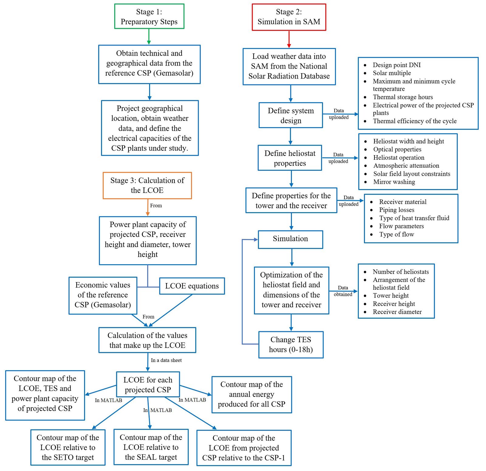
Fig. 1. Three-step methodology used to obtain the LCOE.
2.1. Stage 1: preparatory step
The first stage involved defining the geographical location and technical parameters of CSP-1. Table 1 presents the location in terms of latitude and longitude (northern hemisphere), the electrical power generated, and the area occupied by the CSP-1 plant. This table was also used to specify the location of the projected plants (CSP-2 to CSP-5) in the southern hemisphere, along with their respective generation capacities in megawatts electric (MWe), as shown in Fig. 1. The geographical location is a crucial factor, as it allows for obtaining annual meteorological data on direct radiation specific to each study site, extracted from the National Solar Radiation Database (NSRDB). Table 2 summarizes the technical parameters of CSP-1, which will be used to calculate its LCOE and to scale the associated costs for the projected plants.
Table 1
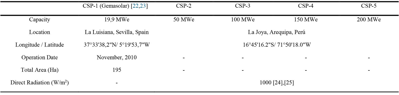
Table 1. General specifications of the CSP plants under study.
Table 2
![Technical values of CSP-1 [17,21,26].](figures/12-51-15.jpg)
Table 2. Technical values of CSP-1 [17,21,26].
Figure 2 presents the basic schematic of CSP-1, showcasing its essential components. The tower, which supports the receiver, is responsible for capturing solar radiation reflected by the field of heliostats, achieving operating temperatures of 590 °C in the tower and 290 °C in the receiver [21]. The heat transfer fluid, which absorbs the heat, is transported to the hot storage tank of molten salts at approximately 565 °C, from where it is then pumped to the steam generator. The generated steam drives the turbine, which operates under a Rankine cycle and is connected to the generator, supported by the electric power generation subsystem (EPGS) to stabilize electricity production. After releasing their heat, the molten salts are pumped to the cold storage tank and subsequently transported back to the receiver at an approximate temperature of 290 °C, thus completing the cycle.
Figure 2
![Basic scheme of CSP-1 (Gemasolar) [22].](figures/12-51-2.jpg)
Fig. 2. Basic scheme of CSP-1 (Gemasolar) [22].
2.2. Stage 2: simulations in SAM
In this stage, based on the information detailed in Fig. 1, the weather data and geographical coordinates of the projected CSP plants (located in La Joya, Arequipa, Peru) were loaded into SAM, with their latitude and longitude specified in Table 1. The weather data, obtained from the NSRDB database, were incorporated into SAM and are presented in Fig. 3.
Figure 3
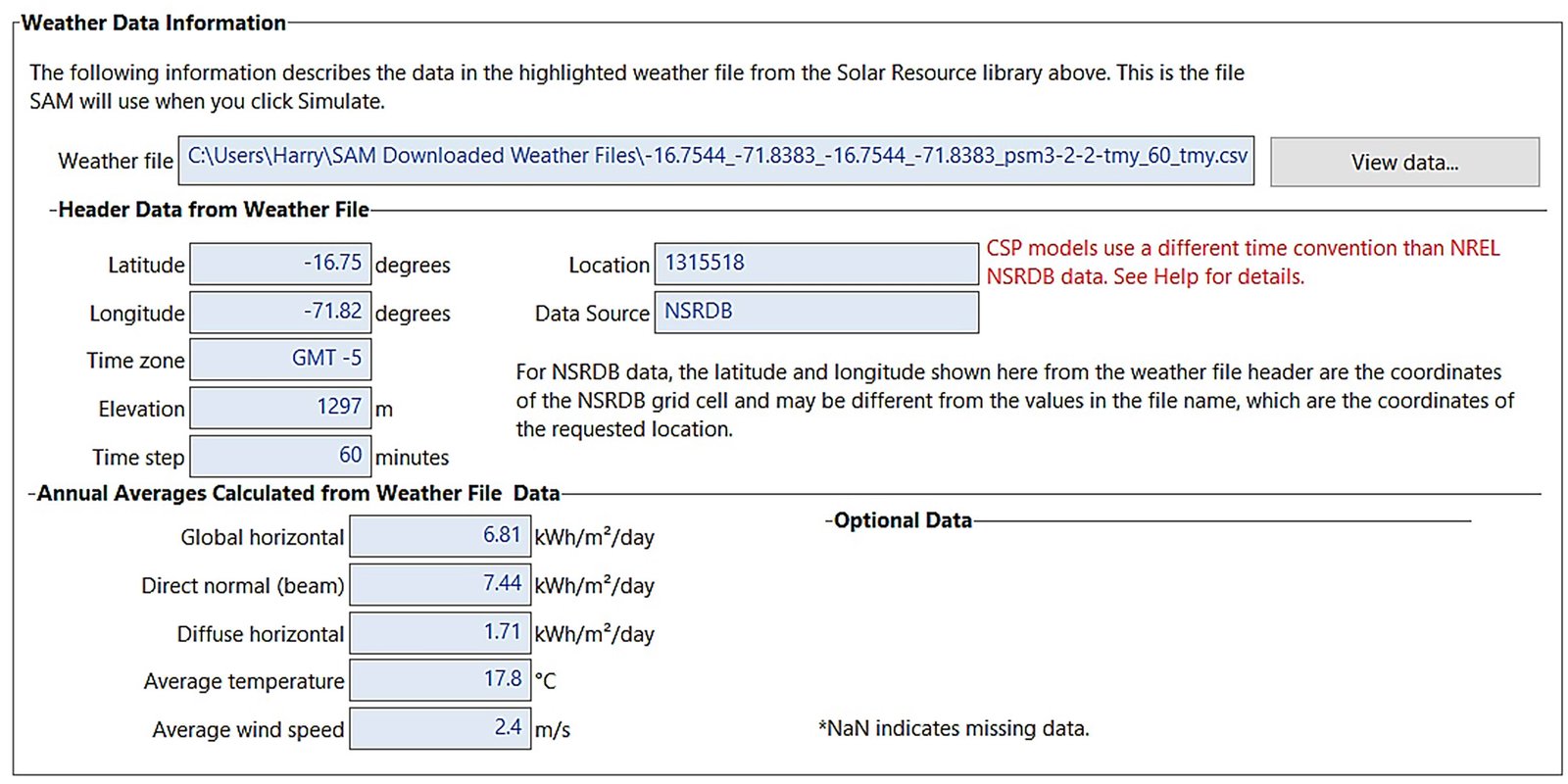
Fig. 3. Weather data information exported to SAM.
After loading the weather data, the design point parameters were defined (Fig. 4). The direct normal irradiation (DNI) was entered according to the data in Table 1, and the solar multiple was set at 1.6, as this value is optimal for achieving maximum efficiency, according to [27]. Values higher than 1.6 do not improve the system's efficiency. The operating temperatures of the tower and the receiver were fixed at 590 °C and 290 °C, respectively, in accordance with the operational values of CSP-1 [21]. In the thermal storage section, values were configured between 0 and 18 hours, while the gross output power of the turbine was set in the range of 50 to 250 MWe.
Figure 4
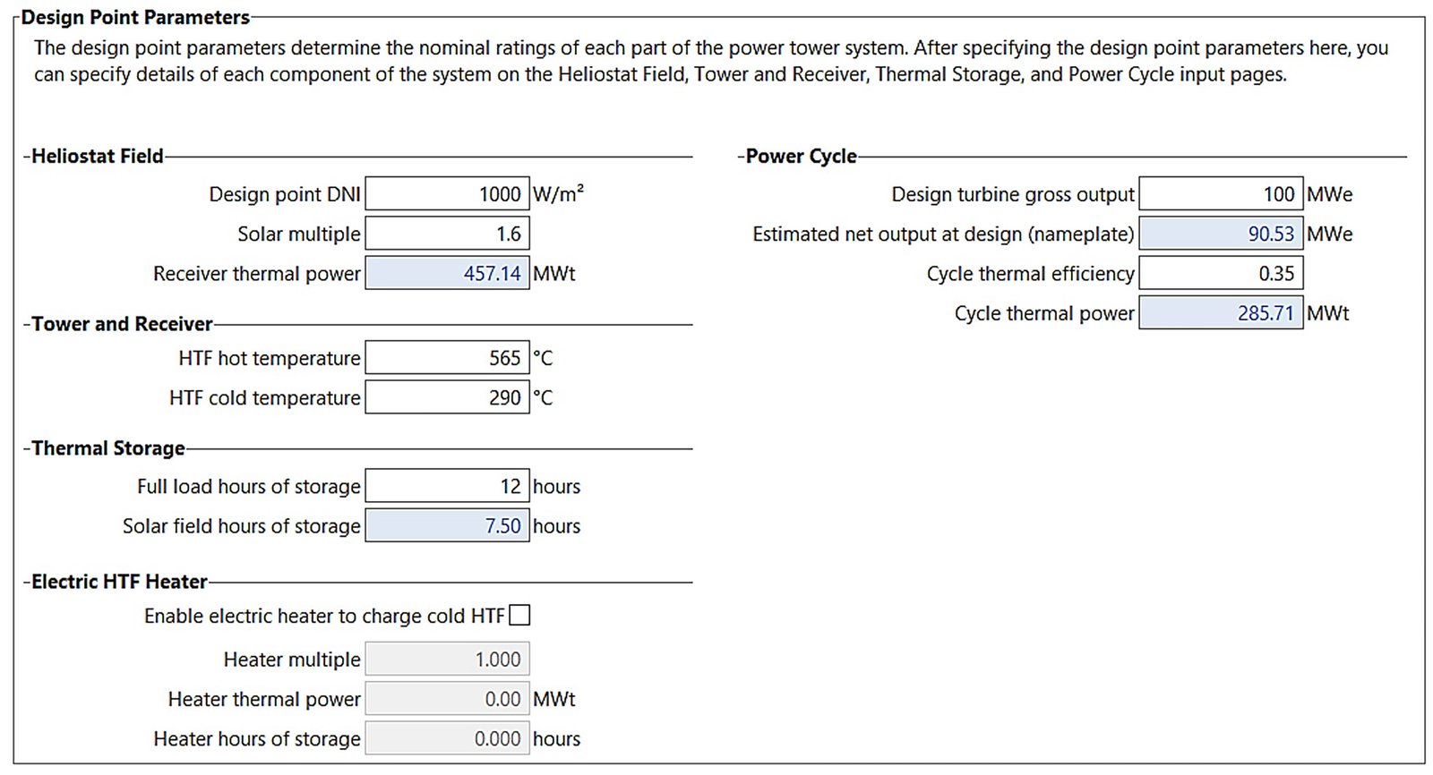
Fig. 4. Design parameters added to SAM.
Once the design point parameters were defined, the heliostat values were established, each reviewed and referenced accordingly, as shown in Table 3. The values entered into SAM are presented in Fig. 5. It is important to note that these values remain constant and were uniformly applied across all simulations of the projected CSP plants.
Table 3
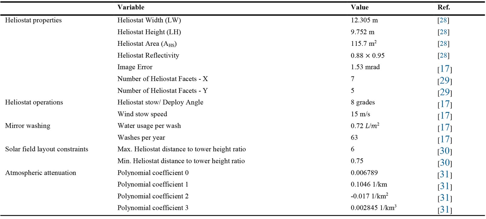
Table 3. Reference Values Set for the Heliostat Field in SAM.
Figure 5
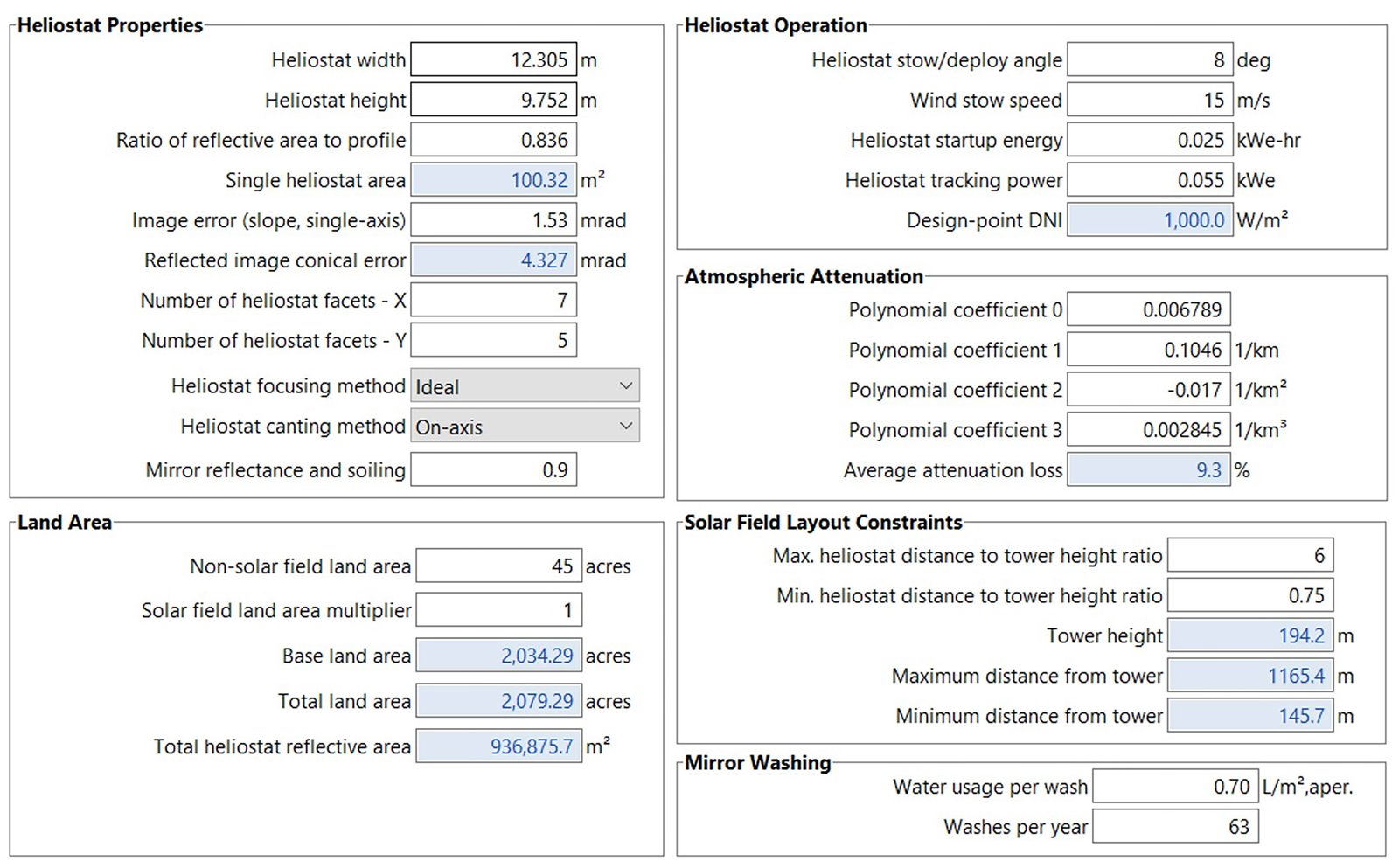
Fig. 5. Reference values entered for the heliostat field in SAM.
The next step was to define the values for the tower and the receiver, including materials, heat transfer properties, heat transfer fluid (HTF), pipe losses, modeling parameters for the flow in the receiver, and design, operational, and flow pattern parameters. These values are presented in Table 4, and their input into SAM is shown in Fig. 6.
Table 4

Table 4. Tower and Receiver Parameters.
Figure 6
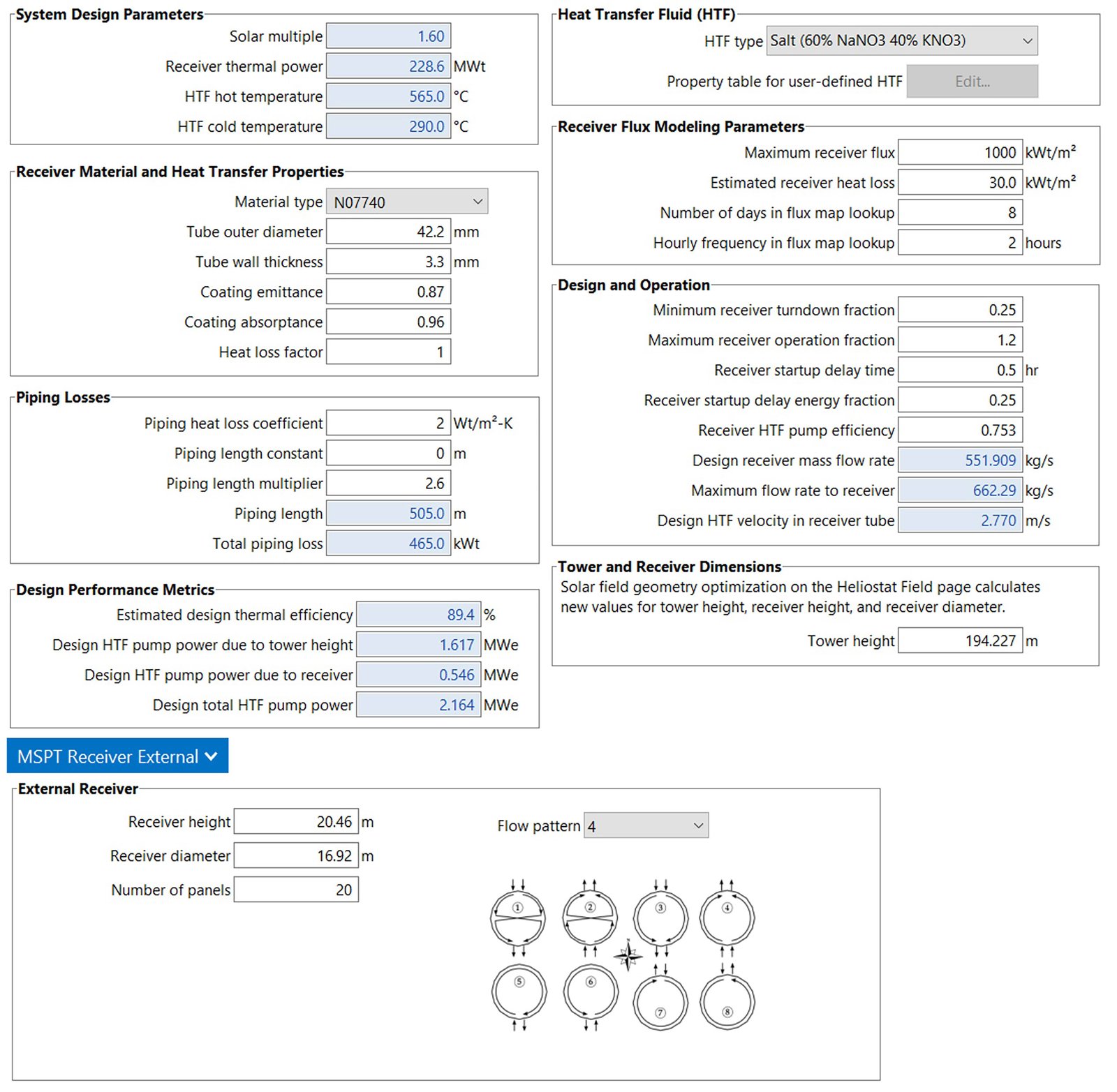
Fig. 6. Loaded parameters for the tower and receiver in SAM.
Finally, the simulation was conducted, as described in Fig. 1 of Stage 2, where 19 simulations were performed by varying the thermal energy storage hours (from 0 to 18 hours of TES) for each projected CSP plant, along with an additional simulation to determine the optimal design. In total, 152 simulations were carried out.
2.3. Stage 3: calculation of levelized cost of energy (LCOE)
To calculate the LCOE, the steps outlined in Fig. 1 of Stage 3 were followed. Based on the power output of the projected CSP plants, as well as the diameter and height of the receiver and the height of the tower obtained in SAM, a scaling economy was applied to project the direct and indirect costs from the reference plant CSP-1, as shown in Table 5 according to [21].
To calculate the various costs, the following equations were used:
Table 5
![Economic values of CSP-1 [21].](figures/12-51-18.jpg)
Table 5. Economic values of CSP-1 [21].
Total land cost: The total land cost \(\left(C_{T-Land}\right)\) will be the cost of the vacant land \(\left(C_L\right)\) in $/m2 and the total area of land occupied by the plant \(\left(A_T\right)\) in m2, as indicated in Eq. (1) [38].
To calculate \(C_L\) it can be determined using the current market value or through Eq. (2) according to [39]. The calculated value is 0.47 $/m2
Total land area: The total land area \(\left(A_T\right)\), is calculated as the product of the heliostat area \(\left(A_H\right)\) and the number of heliostats \(\left(N_H\right)\), multiplied by an additional land factor for the heliostat \(\left(f_{Area-H}=\ 1.92\right)\). This factor is derived from Eq. (3), which represents the relationship between the effective area occupied by the heliostat \(\left(A_{DHS}\right)\) and the reflective area of the heliostat \(\left(A_{HS}\right)\). Additionally, it is increased by 30% to account for pathways and extra land around the field, along with a fixed amount added for the central area of the plant, as detailed in Eq. (2) according to [38]:
Eq. (5) defines the circular area of land occupied by the heliostat \(\left(A_{DHS}\right)\). Equation (6) describes the diameter of the land occupied by the heliostat \(\left(DHs\right)\), which depends on the aspect ratio of the heliostat \(\left(wr\right)\), the safety distance between heliostats \(\left(ds\right)\) and the height of the heliostat \(\left(LH\right)\). Finally, Eq. (7) establishes the relationship between the width (LW) and the height of the heliostat \(\left(LH\right)\). Equations (4)-(7) are described according to [40].
Heliostat cost: The cost of the heliostat \(\left(C_H\right)\), is the price of the heliostat \(\left(P_H\right)\) in dollars per square meter (100 $/m2 according to [41]) multiplied by the area of land occupied by a heliostat \(\left(A_H\ =\ value\ from\ Table\ 3\right)\) as shown in Eq. (8).
Tower cost: The cost of the tower \(\left(C_{TTH}\right)\), is calculated based on the cost of the reference tower \( \left( C_{Tow-ref}=\$ 0.78232\times{10}^6\right)\) and the height of the tower (THT), as shown in Eq. (9) according to [38].
Receiver cost: The cost of the receiver \(\left(C_R\right)\) is calculated based on the cost of the reference receiver \(\left(C_{Rref}=218\ \frac{$}{kWt}\ according\ to\ Table\ 5\right)\) multiplied by the ratio of the area of the study receiver \(\left(A_R,\ value\ calculated\ in\ SAM\right)\) to the area of the reference receiver \(\left(A_{Rref}=300\ m^2\ according\ to\ Table\ 2\right)\), raised to an exponent of 0.8, as shown in Eq. (10) according to [38].
Thermal storage cost: The cost of thermal storage \(\left(C_{MS}\right)\), is calculated as the product of the cost of the reference storage \(\left(C_{MSref}\right)\), as indicated in Table 5, and the thermal energy storage \(\left(Q_{storage}\right)\). The thermal energy storage depends on the projected storage hours \left(h_{TES}\right)\) for Concentrated Solar Power (CSP), as shown in Eq. (11) according to [38]. Additionally, \(Q_{storage}\) is a function of the storage hours \(\left(h_{TES}\right)\), the efficiency of the cycle \(\left(\eta_{cicle}\right)\) and the projected electrical power of the CSP plant \(\left(\dot{W}_{P-plant}\right)\), as indicated in Eq. (12) according to [17].
Power block (BOP) and steam generator (SG) cost: The cost of the balance of plant and steam generator \left(c_{BOP+SG}\right)\), is scaled from the cost of the reference power block \(\left(C_{BOP+SG-ref}\ =\ $\ 37.5\times{10}^6\right)\). This calculation utilizes the ratio of the thermal power at the design point obtained in SAM \(\left(P_{Th-design\ }\right)\), multiplied by the efficiency of the cycle \(\left(\eta_{cicle}=0.35\right)\) and divided by the thermal power of the reference system \(\left(P_{th-ref}\right)\), with a scaling coefficient exponent \(\left(x_{BOP+GV}=0.8\right)\), as indicated in Eq. (13), according to [21] and [38].
Infrastructure costs \(\left(C_{FIXED}\right)\): These costs are estimated independently of the size of the plant, as all plants incur certain common field costs (e.g., buildings, roads, master control system, etc.), as shown in Eq. (14) according to [38]. In this equation, \(\dot{W}_{P-plant}\ \left(W\right)\) represents the electrical power of the turbine at the design point.
Direct costs: Direct costs \(\left(C_D\right)\) correspond to the sum of all previously mentioned costs (cost of the tower, cost of the heliostats, cost of the receiver, cost of thermal storage, and cost of the balance of plant and generator), according to Eq. (15) [42].
Indirect costs: Indirect costs \(\left(C_{ID}\right)\) will be estimated as 12.5% of the direct costs, as there are various indirect costs associated with the construction of a plant, such as contingencies (1 to 2.5% of the direct costs) and management costs (approximately 10% of the direct costs), as indicated in Eq. (16) [42].
Total investment: The total investment is the sum of direct costs \(\left(C_D\right)\) and indirect costs \(\left(C_{ID}\right)\), as indicated in Eq. (17).
Fixed charge rate (FCR): The FCR represents the amount of revenue per unit of investment that a company must generate annually to cover the expenses associated with the depreciation and amortization of that investment. It is calculated using Eqs. (18), (19), and (20), according to [38] and [42]. The values used in these equations are summarized in Table 6.
Table 6
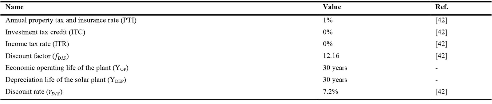
Table 6. Values for calculating the FCR.
The calculated values are \(f_{DIS}=12.16\) (discount factor), allowable depreciation DEP=0.0405 and the fixed charge rate \( FCR=0.0922 \left(9.22\%\right)\).
Operation and maintenance costs \(\left(C_{O \& M}\right)\): These costs are determined by the initial rate \(\left({O \& M}_i\right)\), the annual inflation \(\left(r_{inf}=2.4\%\right)\) [43], the discount rate \(\left(r_{DIS}=7.2\%\right)\), and the economic lifespan of the plant YOP=30 años. The \(C_{O \& M}\) is expressed as a percentage of the total investment, as shown in Eq. (14) [38]. Given that maintenance costs vary considerably, ranging from 6% to 20% of the initial cost according to [44] and [45], a value of 3.5 \(\frac{$}{{MWh}_e}\) was assumed according to [46] and [47], which is multiplied by our annual electricity production \(\left(E_{electric\ anual}\right)\) as indicated in Eq. (22).
2.4. LCOE calculation
Finally, with all the aforementioned data, we can proceed to calculate the Levelized Cost of Energy (LCOE), considering the fixed charge rate (FCR), the total investment (IT), the maintenance costs, and fuel costs (which are not taken into account in this case), as well as the net energy produced by the plant \(\left(E_{electric\ anual\ }\right)\) in kWh, as indicated in Eq. (23) [38] and [42].
3. Results
The results will be presented in four sections:
In Section 3.1, the results for the Levelized Cost of Energy (LCOE) values for the five projected Concentrated Solar Power (CSP) plants, all with 15 hours of thermal energy storage (TES), will be presented. This section will focus solely on the total LCOE value. This decision is based on the fact that CSP-1 is designed to operate with 15 hours of TES, allowing for a fair comparison of LCOE values among the CSP plants. Additionally, the LCOE value will be compared to the SETO target of 5 ¢/kWh for \(TES\geq12\ h\) according to [19], as well as the current value from the electricity supplier SEAL, which is 20 ¢/kWh according to [20]. Other LCOE values for different thermal storage capacities will not be compared due to the completion of 152 simulations. In Section 3.2, the components of the LCOE for 15 hours of TES will be analyzed, along with their percentage contribution by component.
In Section 3.3, the LCOE values for all projected CSP plants will be examined using a contour map. The LCOE values will also be analyzed as a percentage in relation to the SETO target, the value from the local electricity supplier SEAL, and CSP-1.
Finally, in Section 3.4, the annual electricity production for a TES of 15 hours will be analyzed, along with the annual electricity production represented in a contour map for all projected power outputs and TES ranging from 0 to 18 hours.
3.1 Levelized cost of energy for plants with 15 hours of thermal storage
The LCOE values for CSP-2 to CSP-5 in Fig. 7 suggest a higher LCOE compared to the SETO target and a lower LCOE in relation to that of SEAL. In the case of CSP-1, its LCOE value is higher than all the presented values due to elevated costs during its construction year. The figure shows that the LCOE of CSP-1 is four times greater than the SETO value; however, according to [48], the actual LCOE value of CSP-1 in 2020 (28 ¢/kWh) would be 5.6 times greater. For CSP-2, the LCOE is 2.4 times higher than that of SETO; for CSP-3, it is 2.5 times higher; for CSP-4, it is 2.7 times higher; and for CSP-5, it is 3.3 times higher than the SETO value. In the same figure, in relation to the LCOE of SEAL, it is observed that the LCOE of CSP-1 is 1.8% higher than that of SEAL. Meanwhile, CSP-2 has an LCOE that is 40.25% lower than SEAL's, CSP-3 is 37.65% lower, CSP-4 is 31.9% lower, and finally, CSP-5 is 17.85% lower than SEAL's value.
Figure 7
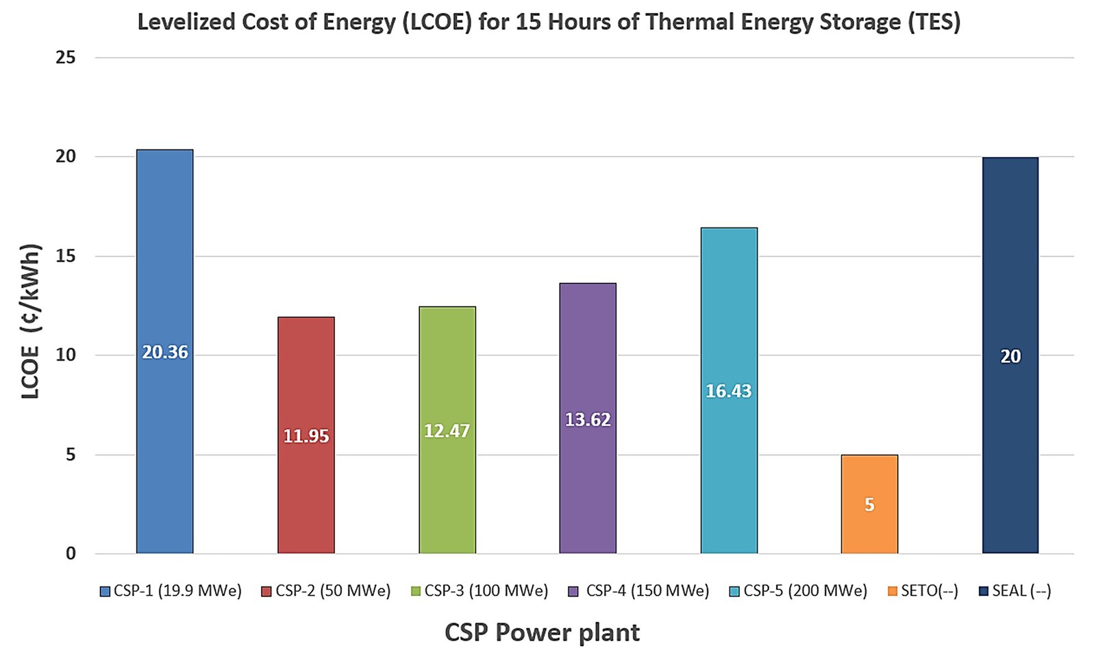
Fig. 7. LCOE values for 15 hours of thermal energy storage (TES).
3.2. Levelized cost of energy for plants with 15 hours of thermal storage by components
In the analysis of LCOE values, it is crucial to understand how costs are distributed by components, as illustrated in Fig. 8. It can be observed that for plants CSP-2 to CSP-5, the costs of heliostats and the receiver have decreased by approximately 45% compared to CSP-1. Additionally, the cost of the balance of plant (BOP) has been reduced by an average of about 69.33%, while the cost of thermal energy storage (TES) has increased by an average of approximately 58.54% compared to CSP-1.
Figure 8
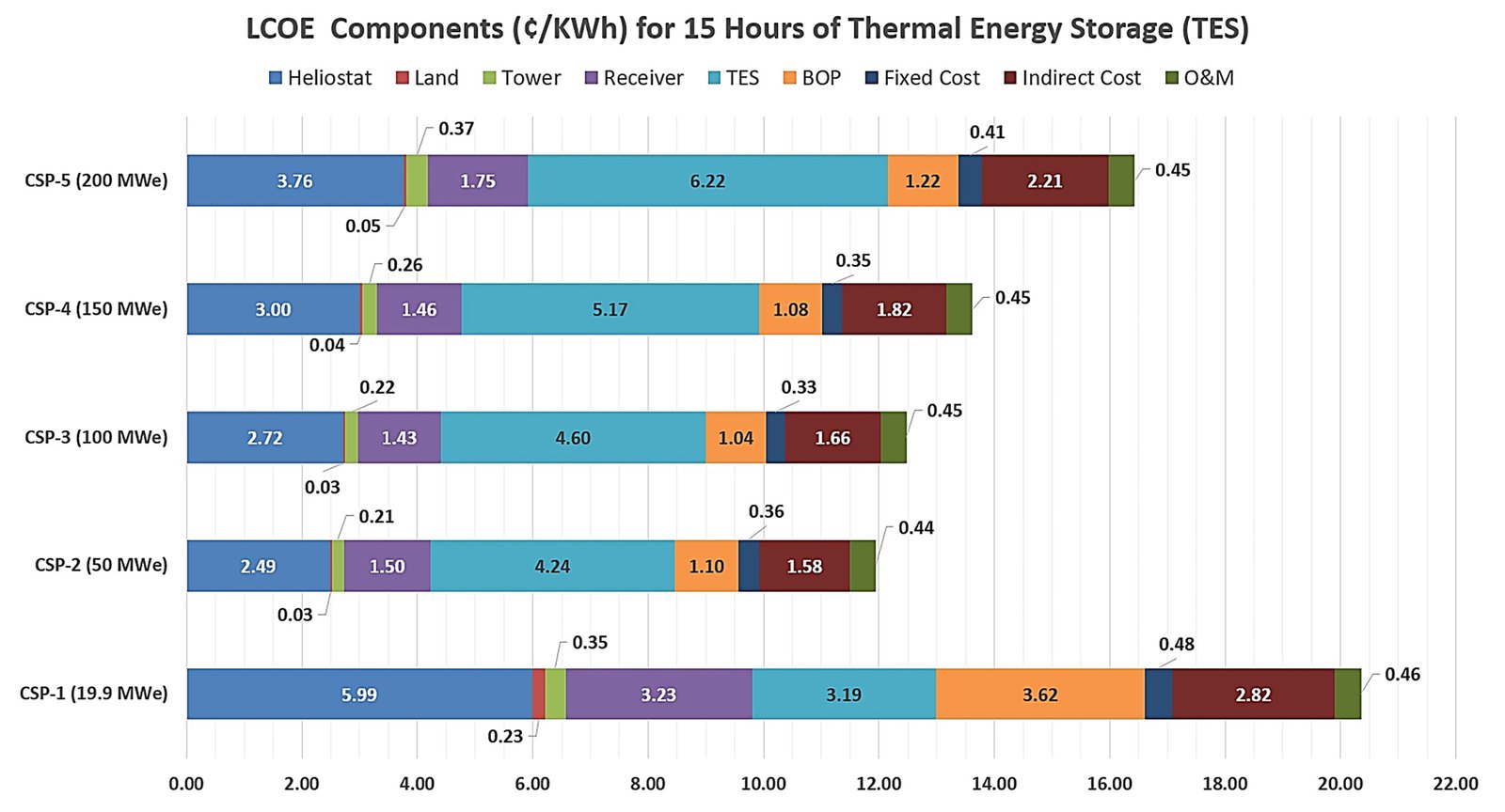
Fig. 8. Components of the LCOE for 15 hours of TES in the CSP plants under study.
Regarding the heliostat component, Fig. 8 shows that costs decrease between 37% and 58.43% from CSP-2 to CSP-4 compared to CSP-1, due to the reduction in costs from $158/m² to $100/m² currently, according to [41].
In relation to the BOP component, Fig. 8 indicates that costs have been reduced to about one-third, with a reduction ranging from 66.3% to 71.2% compared to the value of CSP-1.
Concerning the receiver component, Fig. 8 indicates that the cost reduction from CSP-2 to CSP-4 compared to CSP-1 varies between 45.82% and 55.72%. On the other hand, the TES component of the LCOE shows an increase.
Regarding the TES component, Fig. 8 indicates that the cost increase from CSP-2 to CSP-4 compared to CSP-1 varies between 32.9% and 94.98%. Although this might seem like a disadvantage, it actually represents an advantage, as it allows for a design power output that is 2.5 to 10 times greater with a lower LCOE than that of CSP-1.
With respect to the LCOE component of indirect costs in Fig. 8, the cost reduction from CSP-2 to CSP-4 compared to CSP-1 varies between 21.63% and 43.97%. Fixed costs range from 3% to 2.48%, being slightly higher than those of CSP-1. Finally, operation and maintenance (O&M) costs have drastically decreased, from 1.15% in CSP-1 to 0.28% in the remaining CSP plants.
A detailed analysis of Fig. 9(a), which breaks down the costs that comprise the LCOE by percentage, reveals that in CSP-1, the largest cost corresponds to the heliostats, accounting for 29.4% of the total, followed by the BOP at 17.77%. The receiver ranks third at 15.88%, while thermal energy storage (TES) represents 15.66%. Indirect costs are in fifth place, representing 13.84%. Altogether, 78.71% of the total cost of CSP-1 (16.025 ¢/kWh) is attributed to the heliostats, the balance of plant, the receiver, and thermal storage, reflecting the significant initial project costs (2009) [48].
Figure 9
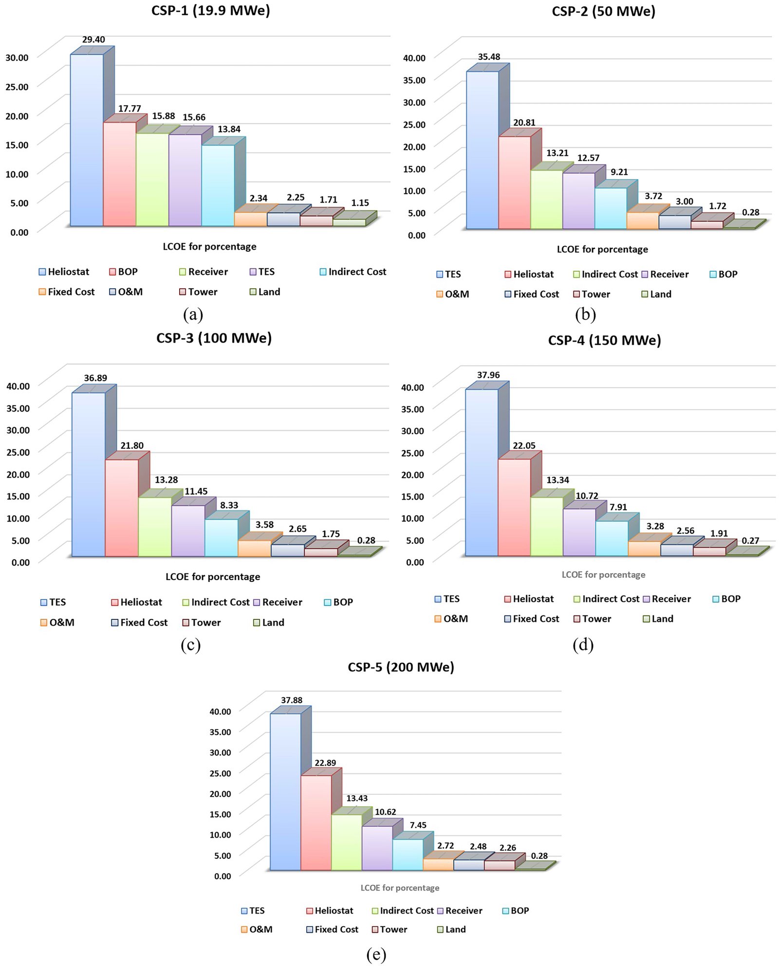
Fig. 9. Percentage components of the LCOE for 15 Hours of TES in the CSP plants under study. (a) CSP-1 in descending order. (b) CSP-2 in descending order. (c) CSP-3 in descending order. (d) CSP-4 in descending order. (e) CSP-5 in descending order.
In Fig. 9(b) to (e), the analysis shows that, on average, 78.6% of the total cost for configurations CSP-2 to CSP-5 is attributed to the same main components: heliostats, BOP, receiver, and TES. In these configurations, the LCOE varies between 9.392 ¢/kWh and 12.914 ¢/kWh, with TES being the largest cost component, followed by heliostats, the receiver, and finally, the BOP.
Figures 10(a)–(d) clearly illustrate the changes in the main costs (TES, heliostats, receiver, BOP) among the different CSP configurations. In Figure 10(a), the percentage of TES as a component of the LCOE is presented, which averages 37.05% for CSP-2 to CSP-5, in contrast to 15.66% for CSP-1. Figure 10(b) shows the average percentage costs of heliostats in CSP-2 to CSP-5, which account for 21.89% of the LCOE, compared to 29.4% for CSP-1. Figure 10(c) illustrates the percentage cost of the BOP, with an average of 8.23% for CSP-2 to CSP-5, compared to 17.77% in CSP-1. Finally, Fig. 10(d) shows the percentage cost of the receiver in CSP-2 to CSP-5, which has an average of 11.34%, compared to 15.88% for CSP-1.
Figure 10

Fig. 10. Percentage analysis of the four most important costs comprising the LCOE for a 15-hour TES. (a) Percentage variation of TES contributing to the LCOE for all CSPs. (b) Percentage variation of the heliostat contributing to the LCOE for all CSPs. (c) Percentage variation of the BOP contributing to the LCOE for all CSPs. (d) Percentage variation of the receiver contributing to the LCOE for all CSPs.
3.3. Levelized cost of energy for all CSPs
To analyze the variations in LCOE across all design capacities of CSP-2 to CSP-5, within a range of 0 to 18 hours of TES, contour maps were created with increments of 50 MWe, reaching up to 200 MWe. It was also necessary to examine the percentage variations in LCOE for each studied CSP in comparison to CSP-1. Additionally, variations in LCOE were investigated within the ranges of 50 MWe to 200 MWe, identifying the minimum LCOE value in each case.
Figure 11(a) presents the LCOE values in cents per kilowatt-hour for capacities ranging from 50 MWe to 100 MWe. The red point indicates the minimum LCOE value, which is 7.84 ¢/kWh and corresponds to a 50 MWe plant with 1 hour of TES. When comparing values with TES ≥ 12 h to the SETO target (5 ¢/kWh), it is observed that the cost exceeds 11 ¢/kWh, indicating that these values are 2.2 to 2.6 times greater than the SETO target.
Figure 11
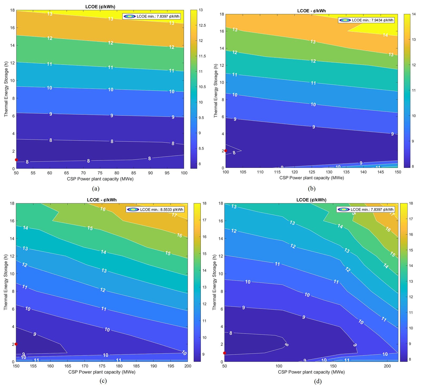
Fig. 11. Variation of the LCOE in ¢/kWh. (a) LCOE between CSP-2 and CSP-3. (b) LCOE between CSP-3 and CSP-4. (c) LCOE between CSP-4 and CSP-5. (d) LCOE between CSP-2 and CSP-5.
Figure 11(b) shows the LCOE values in cents per kilowatt-hour for capacities from 100 MWe to 150 MWe. The red point marks the minimum LCOE value, which is 7.94 ¢/kWh, corresponding to a 100 MWe plant with 2 hours of TES. When comparing values with TES ≥ 12 h to the SETO target (5 ¢/kWh), it is noted that the LCOE exceeds 11 ¢/kWh, suggesting that these values are 2.2 to 2.8 times greater than the SETO target.
Figure 11(c) presents the LCOE values in cents per kilowatt-hour for capacities from 150 MWe to 200 MWe. The red point indicates the minimum LCOE value of 8.55 ¢/kWh, corresponding to a 150 MWe plant with 2 hours of TES. When comparing values with TES ≥ 12 h to the SETO target (5 ¢/kWh), it is observed that the LCOE exceeds 12 ¢/kWh, indicating that these values are 2.4 to 3.6 times greater than the SETO target.
Figure 11(d) presents the LCOE values in cents per kilowatt-hour for the capacities of CSP-2 to CSP-5. By focusing the analysis on the LCOE values for TES ≥ 12 hours, the following observations can be made:
- For CSPs with capacities ranging from 55 MWe to 140 MWe, the LCOE is between 11 ¢/kWh and 12 ¢/kWh for TES = 12 h.
- For CSPs with capacities from 140 MWe to 165 MWe, the LCOE varies between 12 ¢/kWh and 13 ¢/kWh for TES = 12 h.
- For CSPs with capacities from 165 MWe to 182.5 MWe, the LCOE is between 13 ¢/kWh and 14 ¢/kWh for TES = 12 h.
- For CSPs with capacities from 182.5 MWe to 187.5 MWe, the LCOE ranges from 14 ¢/kWh to 15 ¢/kWh for TES = 12 h.
Increasing the TES to 13, 14, or 15 hours would allow the LCOE to fluctuate between 12 ¢/kWh and 15 ¢/kWh, while raising the TES to 16 hours would bring the LCOE into a range of 13 ¢/kWh to 17 ¢/kWh.
Figure 12(a) presents the percentage values relative to the SETO target. It can be observed that for the projected plants from CSP-2 to CSP-5, the costs are between 156% and 360% higher than the SETO target. This disparity is attributed to the high costs associated with the technology used and the reference costs.
Figure 12
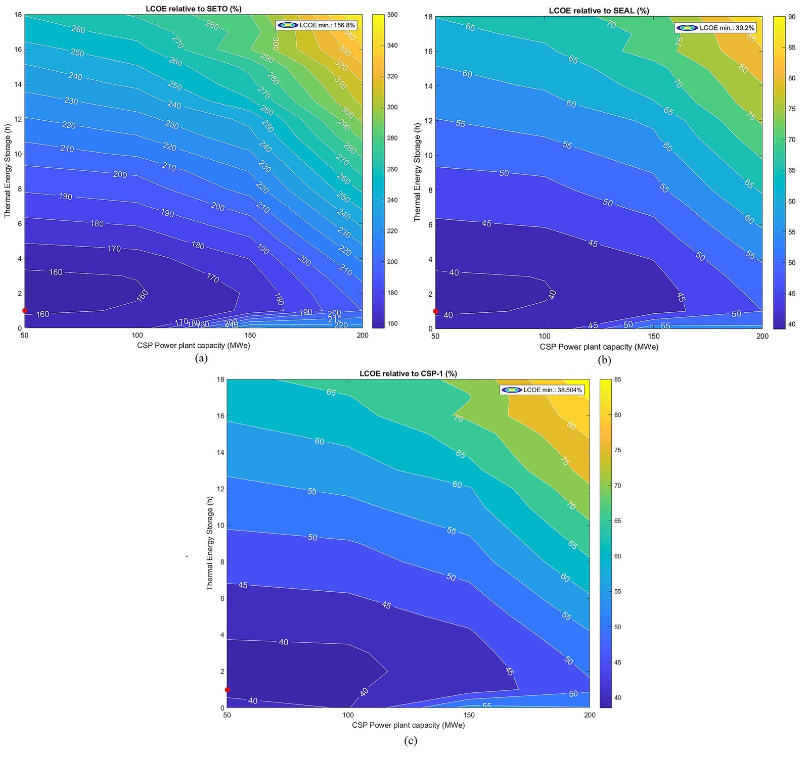
Fig. 12. Percentage values of the LCOE. (a) Relative to SETO. (b) Relative to SEAL. (c) Relative to CSP-1.
In Figure 12(b), the percentage values relative to the local SEAL tariff (20 ¢/kWh) are shown. For the projected plants from CSP-2 to CSP-5, the costs represent between 39% and 90% of the SEAL LCOE, indicating that any power implemented in the city of La Joya would offer electricity below the local tariff.
Figure 12(c) presents the percentage values of the LCOE relative to CSP-1 (20.36 ¢/kWh). It is observed that for the projected plants from CSP-2 to CSP-5, the costs represent between 38.5% and 85% of the LCOE of CSP-1. This indicates a potential maximum reduction of the LCOE of 61.5% for CSPs with a size 2.5 times that of CSP-1, and a 15% reduction for CSPs with a size 10 times greater than that of CSP-1.
3.4. Annual electricity generation for all CSPs
In Fig. 13(a), the annual electrical energy in GWh for 15 hours of thermal energy storage (TES) is presented. It can be observed that as the projected capacity of the concentrated solar power (CSP) system increases, the energy production also increases. Specifically, the energy production of CSP-5 is 5.68 times that of CSP-1, CSP-4 is 5.13 times that of CSP-1, CSP-3 is 3.78 times that of CSP-1, and CSP-2 is 2.07 times that of CSP-1.
Figure 13
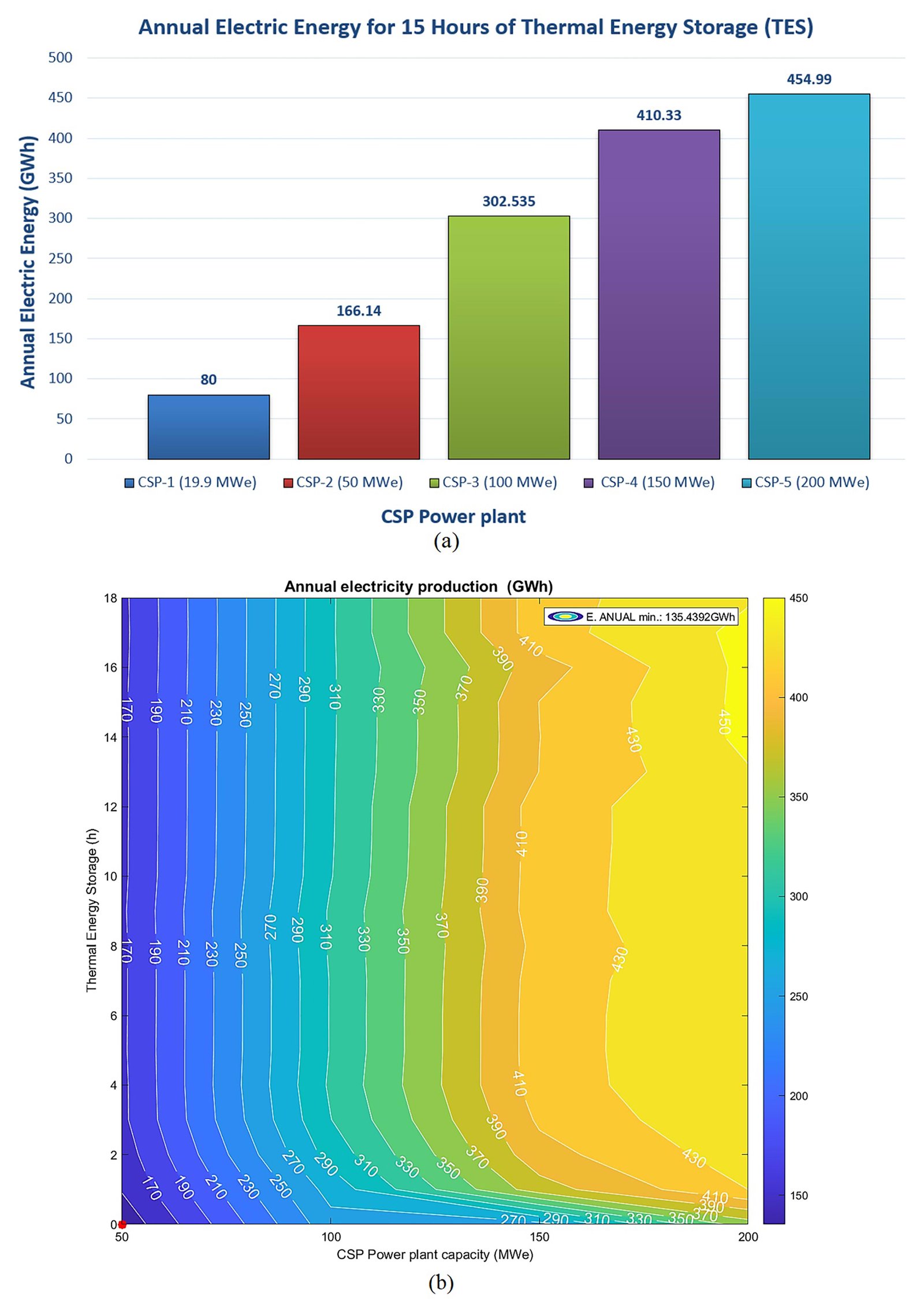
Fig. 13. Annual electricity production (GWh) for all CSPs.
In Fig. 13(b), the annual electricity production in GWh for all projected CSP plants is presented. The values range from 135.43 GWh for CSP-2 (50 MWe) to over 450 GWh for CSP-5. Compared to CSP-1, all projected CSP systems exceed the annual energy production of CSP-1 by a factor ranging from 1.69 to 5.6. Furthermore, it can be observed that annual electricity production increases significantly as capacity rises from 50 MWe to 150 MWe. Specifically, from CSP-2 to CSP-3, the annual electricity production increases by approximately 140 GWh; from CSP-3 to CSP-4, the increase is around 100 GWh; and from CSP-4 to CSP-5, the rise is close to 30 GWh.
4. Discussions
In relation to the study conducted, the following findings can be highlighted:
- The four most significant direct costs that make up the LCOE are thermal energy storage, heliostats, the receiver, and the power block.
- TES is the highest cost within the LCOE, due to the competitiveness that tower solar concentration plants must achieve to surpass the performance of those without it. However, due to current high costs, new technologies are being developed to reduce them, as noted in [49] (Kuravi et al., 2012). The importance of reducing this cost lies in its potential to contribute to a 20% decrease in the LCOE value, according to [49]. If the cost of TES were reduced by 30% (currently $32.7/kWht in this study), our costs could decrease to approximately $22.89/kWht.
- Heliostats are the second most important component in the LCOE. For example, from 2009, when Gemasolar began operations, to 2024 (14 years), the cost of heliostats has decreased by 36.71%, equivalent to an average annual rate of 2.45%. This suggests that costs could reduce from $100/m² to about $85.3/m² by 2030, which is not far from the estimated $75/m² according to [41] (Pfahl et al., 2017).
- The third most significant cost, the receiver, will be affected by improving operating temperatures between 600 and 700 °C and increasing efficiency by 13%, according to [48], resulting in a reduction of 2 ¢/kWh in the total LCOE cost. The receiver costs in individual studies conducted in 2010, such as 'Utility Studies' and 'Abengoa Study', reported values of $71 and $58/kWt, respectively, according to [50]. More recent studies conducted in 2022 establish values of $147/kWt, according to [51]. Compared to the costs of this study ($218/kWt), a reduction of 32.57% is observed, which corresponds to an average annual decrease of 2.17%.
- The fourth most significant cost, the power block, experienced a 40% decrease over 10 years (2010-2020), dropping from $1,499/kWe to $892/kWe, according to [52], with intermediate values of $1,150/kWe in 2015, according to [53] (Kurup et al., 2015). If we estimate the reduction over a 5-year period, from 2010 to 2015, relative to our reference cost ($1,471.5/kWe), the costs fell by 21.85%, which corresponds to an average annual decrease of 4.37%.
By adjusting the recent values (TES, heliostat, receiver, and BOP) from Fig. 7, the LCOE costs for CSP-2 plants decrease from 11.95 to 9.104 ¢/kWh, representing a reduction of 23.82%. For CSP-3, the LCOE costs drop from 12.47 to 9.515 ¢/kWh, equivalent to a reduction of 23.7%. For CSP-4, the LCOE costs decrease from 13.62 to 10.39 ¢/kWh, which represents a decline of 23.72%. Finally, for CSP-5, the LCOE costs reduce from 16.43 to 12.542 ¢/kWh, equivalent to a decrease of 23.66%.
5. Conclusions
From the LCOE values for CSP-2 to CSP-5 plants, it is observed that their costs are between 120% and 260% higher than the SETO target (5 ¢/kWh), with values ranging from 11 ¢/kWh to 18 ¢/kWh. This leads to the conclusion that none of the analyzed CSP plants could achieve this target by the year 2030. By adjusting with recent data, it is estimated that the average percentage reduction in LCOE for 2024 is 23.72%, implying that the LCOE would be between 96.28% and 236.28% above the SETO target. This indicates that, even today, we are still far from achieving that goal.
Based on the analysis of cost reductions in the main components of the LCOE over the past 14 years, it is concluded that the average annual reduction is 1.69%. This suggests that by 2030, an additional estimated reduction of 10.14% could be achieved. With this decrease, the LCOE values would range from 86.28% to 226.28% above the SETO target for CSP plants with capacities between 50 and 200 MWe.
It is concluded that for CSP-2 to CSP-5 plants, the LCOE values in 2024 are between 10% and 61% lower than the current SEAL rate (20 ¢/kWh), falling within a range of 12.2 to 18 ¢/kWh. This suggests that this technology offers more competitive energy costs, which is attractive to both investors and the Peruvian state as an investment opportunity in this type of technology.
According to [54], the LCOE for the Rubí photovoltaic plant (144.5 MWe) in Moquegua, Peru, was 4.79 ¢/kWh in 2018, producing 440 GWh of energy annually. In comparison, our analysis suggests that the LCOE for a CSP plant under the same conditions would be approximately 10.5 ¢/kWh, with 4 hours of thermal energy storage (TES), generating the same annual amount of energy, which represents a 219.2% increase over the Rubí LCOE. Although this value seems less competitive, CSP technology offers significant advantages: it allows for greater flexibility in generation by storing the produced heat and releasing it when economically favorable, provides greater supply stability, and presents higher capacity factors since it can operate more hours per day due to TES. While the capacity factor of the Rubí plant is 33% according to [55], CSP plants achieve capacity factors between 50% and 65%, according to [56].
It can be concluded that the annual electricity production in CSPs shows a significant increasing trend as generation capacity increases, particularly when moving from 50 MWe to 150 MWe. This observation underscores the positive relationship between plant capacity and its electricity production. However, although production continues to increase with each capacity increment, the growth rate diminishes as higher capacities are reached. This is evident in the significant increase of approximately 140 GWh between CSP-2 and CSP-3, compared to the modest increase of about 30 GWh between CSP-4 and CSP-5.
It is concluded that over the past 14 years, LCOE costs for tower CSP plants have decreased significantly. In this analysis, data from CSP-2 to CSP-5, compared to those from CSP-1, show a reduction of 18% to 42.5% in costs, with generation capacities between 2.5 and 10 times greater than the design power of CSP-1, maintaining the same thermal energy storage (TES) of 15 hours.
It is concluded that the components of the LCOE with the greatest impact on costs are thermal energy storage (TES), heliostats, the receiver, and the balance of plant (BOP), which together represent 78.6% of the total LCOE. Of the values obtained, TES accounts for 37.05% of the LCOE cost, followed by heliostats at 21.89%, the receiver at 11.34%, and finally, the BOP at 8.23%. Among these components, TES could contribute to a significant reduction in the LCOE cost, with a potential reduction of 20% [49]. However, phase change material encapsulation technologies are currently in an experimental stage.
Declaration of competing interest
The authors declare no conflict of interest.
References
- Energía - Desarrollo Sostenible. [Online]. Available: https://www.un.org/sustainabledevelopment/es/energy/ (accessed Jul. 24, 2024).
- I. Al-Adwan, M. Al-Hayek, A. A. Issa, M. A. Al Shawabkeh, and Q. Jaber, Using Matlab for simulating real-world photovoltaic system, Jordan Journal of Mechanical and Industrial Engineering, 13 (2019) 21-25.
- J. Lange, J. Hilgedieck, and M. Kaltschmitt, Renewable resources of energy for electricity generation-development trends and necessities within the overall energy system, Jordan Journal of Mechanical and Industrial Engineering, 13 (2019) 207-220.
- J. O. Jaber, M. O. Awadi, A. S. Dalabeeh, and I. M. Mansour, Performance and Socioeconomics of 1st Wheeling PV Project Connected to Medium Grid in Jordan, Jordan Journal of Mechanical and Industrial Engineering, 16 (2022) 567-579.
- G. Cáceres, N. Anrique, A. Girard, J. Degrève, J. Baeyens, and H. L. Zhang, Performance of molten salt solar power towers in Chile, Journal of Renewable and Sustainable Energy, 5 (2013) 053142. https://doi.org/10.1063/1.4826883
- Y. Hu, Z. Xu, C. Zhou, J. Du, and Y. Yao, Design and performance analysis of a multi-reflection heliostat field in solar power tower system, Renewable Energy, 160 (2020) 498-512. https://doi.org/10.1016/j.renene.2020.06.113
- G. M. Tashtoush and M. A. Alzoubi, An analysis of the Performance and Economic Feasibility of a Hybrid Solar Cooling System that Combines an Ejector with Vapor Compression Cycles, Powered by a Photovoltaic Thermal (PV/T) Unit, Jordan Journal of Mechanical and Industrial Engineering,17 (2023) 41-54. https://doi.org/10.59038/jjmie/170104
- H. Al Tahaineh and W. Hassan, Simulation-Design and Performance Analysis of a Small-Scale Concentrating Solar Parabolic Dish System for Hot Water Generation, Jordan Journal of Mechanical and Industrial Engineering, 17 (2023) 413-419. https://doi.org/10.59038/jjmie/170310
- M. T. Zamani and A. A. Amiri, Energy efficiency in smart schools using renewable energy strategy, Journal of Daylighting, 11 (2024) 203-215. https://doi.org/10.15627/jd.2024.15
- Q. He, H. Zheng, X. Ma, and G. Wang, Optical analysis of a sliding-type cylindrical Fresnel lens concentrating collector for agricultural greenhouse, Journal of Daylighting, 8 (2021) 110-119. https://doi.org/10.15627/jd.2021.8
- J. Jiang, M. Moallem, and Y. Zheng, An intelligent iot-enabled lighting system for energy-efficient crop production, Journal of Daylighting, 8 (2021) 86-99. https://doi.org/10.15627/jd.2021.6
- H. Ait Lahoussine Ouali, M. I. Soomro, S. Touili, M. Eltaweel, and A. Alami Merrouni, Performance investigation of seawater desalination system powered by central receiver concentrated solar thermal plant, Applied Thermal Engineering, 225 (2023). https://doi.org/10.1016/j.applthermaleng.2023.120165
- X. Ma, H. Zheng, and S. Liu, A review on solar concentrators with multi-surface and multielement combinations, Journal of Daylighting, 6 (2019) 80-96. https://doi.org/10.15627/jd.2019.9
- K. M. Bataineh and A. Gharaibeh, Optimization analyses of parabolic trough (CSP) plants for the desert regions of the middle east and North Africa (MENA), Jordan Journal of Mechanical and Industrial Engineering, 12 (2018) 33-43.
- A. M. Jawarneh, A. K. AL-Migdady, A. K. Ababneh, H. M. Tlilan, and M. Tarwaneh, Measurement and Assessment of Solar Energy in Zarqa Governorate - Jordan, Jordan Journal of Mechanical and Industrial Engineering, 17 (2023) 605-615. https://doi.org/10.59038/jjmie/170415
- Osinergmin, Energías Renovables: Experiencia y Perspectivas en la Ruta del Perú Hacia la Transición Energética. 2019.
- J. J. Ditta Granados, Estudio de viabilidad de un sistema termosolar de receptor central para la generación de energía eléctrica en La Guajira, Colombia, Universidad Carlos III de Madrid, 2018.
- U. Desideri and P. E. Campana, Analysis and comparison between a concentrating solar and a photovoltaic power plant, Applied Energy, 113 (2024) 422-433. https://doi.org/10.1016/j.apenergy.2013.07.046
- Concentración de Energía Solar-Térmica | Departamento de Energía. [Online]. Available: https://www-energy-gov.translate.goog/eere/solar/concentrating-solar-thermal-power?_x_tr_sl=en&_x_tr_tl=es&_x_tr_hl=es&_x_tr_pto=sc (accessed Jul. 26, 2024).
- TarifasSeal - Todos los documentos. [Online]. Available: https://www.seal.com.pe/clientes/TarifasSeal/Forms/AllItems.aspx (accessed Aug. 19, 2024).
- A. L. Avila-Marin, J. Fernandez-Reche, and F. M. Tellez, Evaluation of the potential of central receiver solar power plants: Configuration, optimization and trends, Applied Energy, 112 (2013) 274-288. https://doi.org/10.1016/j.apenergy.2013.05.049
- Gemasolar - Exera Energía. [Online]. Available: https://www.exeraenergia.es/gemasolar/ (accessed Jul. 27, 2024).
- Fuentes de Andalucía - Energías renovables - Tierra de Contrastes. [Online]. Available: https://turismocomarcaecija.com/energias-renovables/ (accessed Jul. 27, 2024).
- H. A. Yapu Maldonado, Diseño de una planta termosolar de receptor central de 100 MWe con almacenamiento en sales fundidas , 2018. [Online]. Available: http://renati.sunedu.gob.pe/handle/sunedu/601398
- A. R. B. Toma, Estudio de viabilidad técnica y económica de un sistema fotovoltaico autónomo en las instalaciones de la UCSP, Repositorio UCSP, p. 119, 2017, [Online]. Available: https://core.ac.uk/download/pdf/225489954.pdf
- D. E. E. Solar, Gemasolar : 24 horas de energía solar Cliente : Torresol Energy, 2011, pp. 2-4
- C.-J. Winter, R. . Sizmann, and L. L. Vant-Hull, Eds., Solar Power Plants, 1st ed. Springer Berlin Heidelberg, 1991. https://doi.org/10.1007/978-3-642-61245-9
- F. J. Collado and J. Guallar, A review of optimized design layouts for solar power tower plants with campo code, Renewable and Sustainable Energy Reviews, 20 (2012) 142-154. https://doi.org/10.1016/j.rser.2012.11.076
- J. I. Burgaleta, S. Arias, and D. Ramirez, Gemasolar, the first tower thermosolar commercial plant with molten salt storage, Solarpaces, (2011) 1-8.
- W. B. Stine and R. W. Harrigan, Solar Energy Fundamentals and Design: With Computer Applications, Ilustrada. 1985.
- F. Biggs and C. N. Vittitoe, The Helios model for the optical behavior of reflecting solar concentrators. Springfield, 1979. https://doi.org/10.2172/6273705
- P. K. Falcone, A handbook for solar central receiver design. Livermore, California: Sandia National Labs., Livermore, CA (USA), 1986. https://doi.org/10.2172/6545992
- M. R. Rodríguez-Sánchez, On the design of solar external receivers, Universidad Carlos III de Madrid, 2015. [Online]. Available: https://core.ac.uk/download/pdf/44309378.pdf
- Tower and Receiver. [Online]. Available: https://samrepo.nrelcloud.org/help/iph_mspt_tower_receiver.html (accessed Jul. 30, 2024).
- Calculation of heat loss from pipes. [Online]. Available: https://www.ter-en.com/en/calculation/poteri_tepla_trub (accessed Jul. 29, 2024).
- A. B. ZAVOICO, Solar Power Tower Design Basis Document, Revision 0, United States, 2001. https://doi.org/10.2172/786629
- C. Frantz, M. Ebert, B. Schlögl-Knothe, M. Binder, and C. Schuhbauer, Experimental Receiver Setup of a High Performance Molten Salt Test Receiver System, in AIP Conference Proceedings, 2023. https://doi.org/10.1063/5.0148772
- B. L. Kistler, A user's manual for DELSOL3: A computer code for calculating the optical performance and optimal system design for solar thermal central receiver plants, United States, 1986. https://doi.org/10.2172/7228886
- Resolución Ministerial N.° 172-2016-Vivienda - Normas y documentos legales - Ministerio de Vivienda, Construcción y Saneamiento - Plataforma del Estado Peruano. [Online]. Available: https://www.gob.pe/institucion/vivienda/normas-legales/12700-172-2016-vivienda (accessed Sep. 23, 2023).
- F. J. Collado, Preliminary design of surrounding heliostat fields, Renewable Energy, 34 (2009) 1359-1363. https://doi.org/10.1016/j.renene.2008.09.003
- A. Pfahl et al., Progress in heliostat development, Solar Energy, 152 (2017) 3-37. https://doi.org/10.1016/j.solener.2017.03.029
- M. Dr. Romero Alvarez, Dimensionamiento y análisis de producción anual de un sistema de receptor central, Master en Energías Renovables y Mercado Energético 2007/2008, 2008. pp. 66, [Online]. Available: https://static.eoi.es/savia/documents/componente45289.pdf
- Perú | Fuerte descenso de la inflación en mayo y se ubica en el centro del rango meta | BBVA Research. [Online]. Available: https://www.bbvaresearch.com/publicaciones/peru-fuerte-descenso-de-la-inflacion-en-mayo-y-se-ubica-en-el-centro-del-rango-meta/ (accessed Aug. 06, 2024).
- B. Hoffschmidt et al., Concentrating solar power, 2012. https://doi.org/10.1016/B978-0-08-087872-0.00319-X
- Concentrating Solar Power | Electricity | 2021 | ATB | NREL. [Online]. Available: https://atb.nrel.gov/electricity/2021/concentrating_solar_power (accessed Aug. 08, 2024).
- O. Behar, D. Sbarbaro, and L. Morán, A practical methodology for the design and cost estimation of solar tower power plants, Sustainability (Switzerland), 12 (2020) 1-16. https://doi.org/10.3390/su12208708
- Concentrating Solar Power | Electricity | 2023 | ATB | NREL. [Online]. Available: https://atb.nrel.gov/electricity/2023/concentrating_solar_power (accessed Aug. 09, 2024).
- Gemasolar Thermosolar Plant / Solar TRES | Concentrating Solar Power Projects | NREL. [Online]. Available: https://solarpaces.nrel.gov/project/gemasolar-thermosolar-plant-solar-tres (accessed Aug. 12, 2024).
- S. Kuravi et al., Thermal Energy Storage for Concentrating Solar Power Plants, Technology & Innovation, 14 (2012) 81-91. https://doi.org/10.3727/194982412X13462021397570
- G. J. Kolb, C. K. Ho, T. R. Mancini, and J. A. Gary, Power tower technology roadmap and cost reduction plan, 2012.
- C. Augustine, D. Kesseli, and C. Turchi, Technoeconomic cost analysis of NREL concentrating solar power Gen3 liquid pathway, in AIP Conference Proceedings, 2022. https://doi.org/10.1063/5.0085836
- Cost of Concentrated solar power (CSP) projects fell from USD 0.38/kWh to USD 0.118/kWh - a decline of 69% - HeliosCSP - Portal de noticias de energía termosolar. [Online]. Available: https://helioscsp.com/cost-of-concentrated-solar-power-csp-projects-fell-from-usd-0-38-kwh-to-usd-0-118-kwh-a-decline-of-69/# (accessed Aug. 17, 2024).
- P. Kurup and C. S. Turchi, Parabolic Trough Collector Cost Update for the System Advisor Model (SAM), 2015. https://doi.org/10.2172/1227713
- J. Arredondo and M. Ramos, Subastas en Plantas de Energía Solar Fotovoltaica y la Paridad de Red en el Perú, Tecnia, 30 (2020) 27-32. https://doi.org/10.21754/tecnia.v30i2.567
- SIEE, "Sistema interactivo de eficiencia energética." [Online]. Available: https://eficienciaenergetica.minem.gob.pe/Content/fileman/Uploads/Documents/boletin/boletin 2020/ (accessed Nov. 03, 2024).
- R. Musi et al., Techno-economic analysis of concentrated solar power plants in terms of levelized cost of electricity, AIP Conference Proceedings, 1850 (2017) 160018. https://doi.org/10.1063/1.4984552
Copyright © 2025 The Author(s). Published by solarlits.com.

3852
Total views
Citations
SHARE ON


