Evaluation of Daylight Availability for Energy Savings

^a Department of Industrial Engineering, University of Naples Federico II. Piazzale Tecchio 80, 80125 Naples, Italy.
^b Department of Energy, Information Engineering and Mathematical Models, University of Palermo. Viale delle Scienze Ed.9, 90128 Palermo, Italy.

* Corresponding author. Tel: +39-081-2538778
laura.bellia@unina.it (L. Bellia)
francesca.fragliasso@unina.it (F. Fragliasso)
alessia.pedace@unipa.it (A. Pedace)

History: Received 23 December 2014 | Revised 25 February 2015 | Accepted 2 March 2015 | Published online 5 March 2015

Citation: Laura Bellia, Francesca Fragliasso, and Alessia Pedace, Evaluation of Daylight Availability for Energy Savings, Journal of Daylighting 2 (2015) 12-20. http://dx.doi.org/10.15627/jd.2015.2

Figures and tables

Figure 1
Table 1
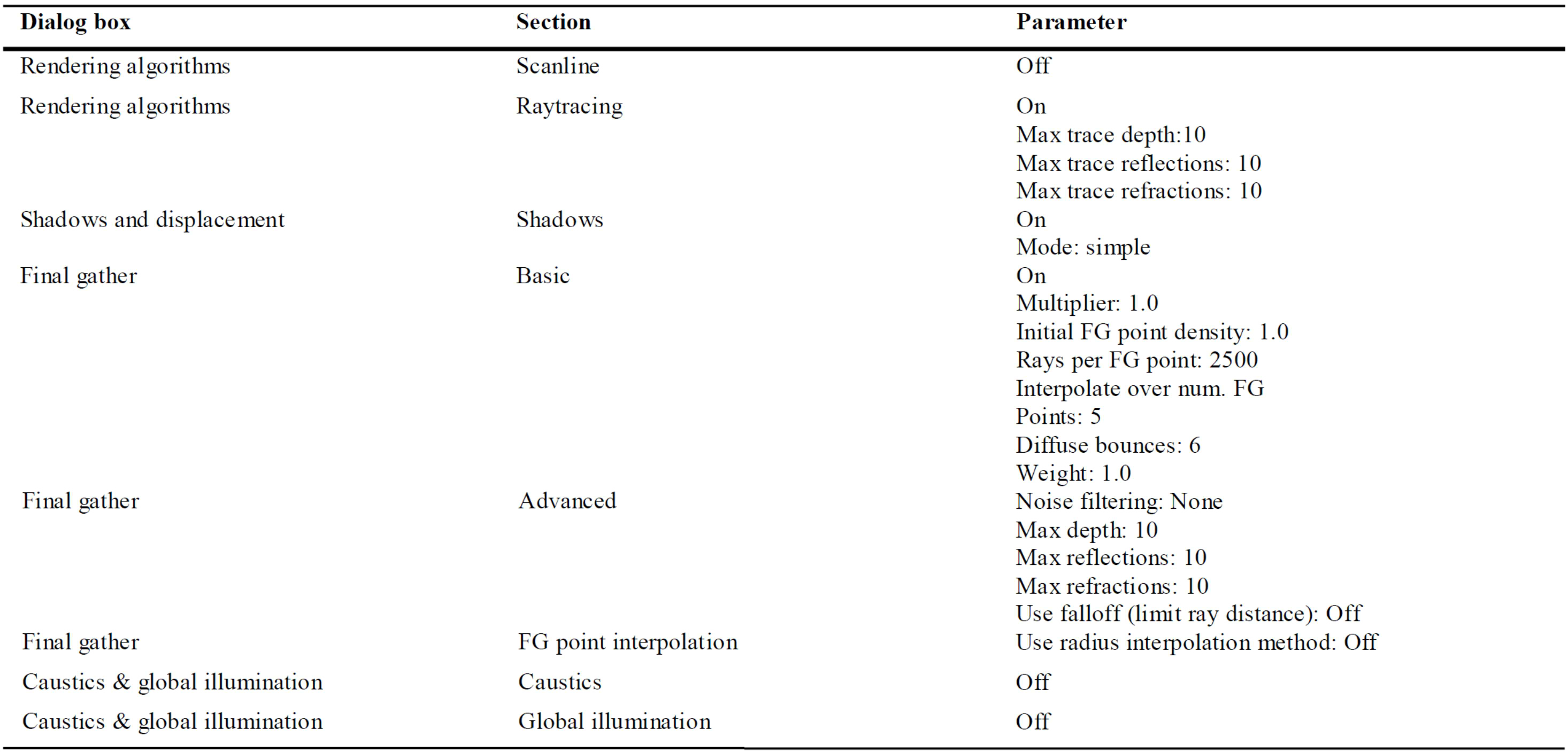Table 2
Figure 2
Table 3
Table 4
Table 5
Figure 3
Figure 4
Table 6
Table 7

Abstract

Dynamic daylight simulations are very useful instruments in daylighting design process. They allow an in depth analysis of indoor daylight availability levels and define if they are adequate to perform a particular visual task. Their results can be used to design shading devices or lighting control systems and compare different technical solutions. The use of these simulations is likely to spread in the common design practice since some regulations and green building rating systems suggest their use. This paper presents dynamic daylight simulation results related to an open-plan office, performed with Autodesk 3ds Max Design^®, which is a calculation software validated by recent researches. It is not used in academic context but it is very widespread between technicians for photorenderings production purposes. The goal of this research is to demonstrate the functionality of this software also in dynamic daylight simulations field and propose an analysis' methodology to use it.

Keywords

Daylighting; Simulation; Shadings; Controls

1. Introduction

The growing need to reduce buildings' energy costs pushes the research towards the experimentation of constantly new solutions for systems' energy efficiency. Daylighting design has a key role in the reduction of energy waste since it allows to maximize the use of daylight in indoor environment and to reduce electric light demand.

The evaluation of daylight availability is not an easy task, since daylight levels in indoor environments can vary depending on many factors: building's location (latitude and longitude) and orientation, day of month and time of day, sky cover, room's geometric and optical characteristics, windows' and glazings' typology, and presence of shadings or external obstructions.

Current research criticizes the daylight calculation static approach based on Daylight Factor (DF) and proposes the dynamic one based on the performing of dynamic daylight simulations [1,2]. Indeed traditional static evaluation approach, based on the use of overcast sky, does not consider the impact of the variation of luminance distribution of the sky, the direct sunlight, and the room orientation [3]. On the contrary dynamic daylight simulations are complex calculation techniques that allow to evaluate, hour by hour during an entire year, illuminance levels inside a built space, by taking into account variable climatic conditions, luminous interreflections between the rooms' surfaces, and the presence of external obstructions.

Dynamic daylight simulations are divided in a series of rather complex phases. The first phase consists in “building” a virtual model that includes all the geometric and optical characteristics of the analyzed space. Then an occupancy profile has to be selected in order to establish during which hours of the year the environment is supposed to be occupied (e.g., in the case of an office, all the hours outside the working time will be excluded from the calculation). At this point a calculation grid has to be determined: is constituted by a series of points for which it is necessary to know the variation of daylight-related illuminance levels during the year (e.g., in the case of a school, each calculation point should be placed in correspondence of students' desks or of the teacher's one). To calculate illuminance levels for each hour of the year related to the calculation grid, it will be necessary to dispose of the climatic data referred to the studied location. Indeed the software is capable of reading the basic climatic data related to global and diffuse irradiance; converting irradiance data into illuminance ones using a luminous efficacy model; generating the sky luminance distribution through sky model; using the sky luminance distribution to calculate indoor illuminances [4].

Simulation's output data are illuminance values corresponding to each calculation point for each hour of the year included in the occupancy profile. For example, in the case of an office with a working schedule of eight hour each day, there are about 2520 working hour in a year excluding holidays. Therefore, the result of the simulation will be 2520 illuminance values for each calculation point.

All these information are difficult to manage, and they have to be summarized to be useful for the technician in the design phase. For this purpose, the so called dynamic daylight performance metrics were introduced. They are performance indicators, which are used to synthesize in a single numeric value the data obtained from dynamic simulations. The most used indicators that were proposed by researchers are: Daylight Autonomy (DA), Continuous Daylight Autonomy (DA_con), Maximum Daylight Autonomy (DA_max), Useful Daylight Illuminance (UDI).

The concept of DA was introduced for the first time in the CIE Daylight Technical Report [5], and it was proposed again in 2001 by Reinhart and Walkenhorst [6] as the annual percentage of the occupied time of a space during which the minimum illuminance indicated by standards is achieved only with daylight. In 2006, Rogers [7] extended the DA and introduced the DA_con. It is calculated as the ratio between the illuminance determined only by daylight on a point and the minimum illuminance required on the workplane required by the standards. For example, if an illuminance equal to 400 lx is registered and the minimum illuminance on the workplane is equal to 500 lx, the DA_con will be 0.8. The DA_max was introduced by Rogers himself in 2006 [7] to consider discomfort risks depending on excessive light levels. The DA_max can be defined as the annual percentage of time during which a maximum illuminance level is trespassed and over which visual discomfort may occur. This limit is set at 10 times the minimum illuminance on the workplane defined by the regulation. For example, if the law establishes 150 lx on the workplane, this limit will be equal to 1500 lx.

The UDI was proposed by Mardaljevic and Nabil in 2005 [8]. It is the result of a series of researches carried out at the Lawrence Berkeley National Laboratory on offices' users. These studies demonstrated that not all the users define as comfortable the same lighting conditions, but generally a range for which all the subjects judged daylight levels as insufficient (below 100 lx) or too intense, and therefore uncomfortable (over 2000 lx) can be identified. The illuminance included in the range of 100-2000 lx was therefore defined as “useful” i.e. helpful to perform the visual task. Consequently, UDI have to be calculated as the percentage of time in a year during which the illuminance registered in a point on the workplane is included in this range from 100 to 2000 lx. In 2006, Mardaljevic proposed a new articulation of the range 100-2000 lx dividing it in two further intervals defined as UDI_{supplementary} (100-500 lx) and as UDI_autonomous (500-2000 lx) in order to account also for the design illuminance established by the regulation (which is equal to 500 lx for offices). If illuminances registered in a point range in the first interval, even though light levels can be judged as sufficient to carry out visual tasks, the integration with electric light is necessary to reach the legislative minimum; if instead they are comprised in the second range, daylight alone is able to guarantee visibility conditions. In short, studying an environment in terms of UDI means to register daylight related illuminances in each analysis point of the studied environment and to verify for each one of them, what are the percentages of time during which they are comprised in four different intervals: under 100 lx, between 100 and 500 lx, between 500 and 2000 lx and over 2000 lx. In the end, it has to be pointed out that 500 lx is the minimum illuminance value on the workplane established by the standards for offices. If the studied environment should be used for a different activity, a different limit for this interval has to be considered.

Specific software is necessary to perform dynamic daylight simulations. Considering research applications, Daysim is the most widespread of them and its daylight calculation model is based on daylight coefficient approach [9]. It is a daylighting analysis tool that allows to evaluate indoor daylight levels, calculate daylight performance indicators, mimic user's interaction whit shading devices and lighting controls, and estimate lighting energy consumptions. Daysim success in academic context depends not only on its features but also on the fact that it uses Radiance engine, “one of the few models validated extensively” [6,10–14].

Another software that allows to perform dynamic daylight simulations is Autodesk 3ds Max Design^®. It uses mental ray engine and it is very widespread in design practice for photo-renderings production purposes but not in research applications. However a recent study by Reinhart and Breton [15] compared indoor daylight levels calculated with Daysim, 3ds Max Design^®, and real measured illuminance data. It was demonstrated that both software produce similar results.

From what has been reported it is clear that the use of these indicators and in general of dynamic simulations is very useful in design practice. Using a dynamic simulation, it is possible to calculate the percentage of time in a year during which discomfort conditions caused by daylight related glare may occur, in order to identify the most appropriate solar shading system to limit this risk; to determine in which way the shading modifies daylight entrance and if it makes necessary the use of electric light; to establish for each calculation point in what percentage daylight fulfills the minimum illuminance values required by the regulations and calculate the percentage of integration with electric light; to estimate daylight distribution and to understand how to design the lighting system's control groups.

For these reasons, current research is very interested in problems connected to dynamic daylight simulations. Above the already mentioned studies about software validations, researchers analyzed different aspects connected to simulations: calculation affecting factors as sky model or weather data file [16–18], the correct modeling of complex materials or fenestration systems [6,14], the uncertainty of users' behavior [19], and the daylight-linked control modeling [20–23].

Furthermore, the potentialities of these dynamic calculation approaches are evident that it is recommended by some regulations and “green building rating systems”. In more detail, the IESNA introduced the concept of Spatial Daylight Autonomy (sDA) and of Annual Sunlight Exposure (ASE) [24]. The USGBC has then included these two parameters in the LEED protocol [25].

sDA indicates the percentage of the workplane for which it occurs that the task illuminance (i.e. 500 lx in the case of offices) is achieved using daylight during 50% of the working hours in a year, whereas ASE indicates the percentage of the workplane for which it occurs that illuminance levels related only to the direct component of daylight exceed the value of 1000 lx for at least 250 hours in a year.

Given these premises, it is clear that dynamic daylight simulations are likely to became popular also in common design practice. As already mentioned, a calculation software like Daysim provides a lot of useful features for daylighting design but it is not very widespread between technicians. On the contrary, 3ds Max Design^® is more widespread but presents some calculation limitations (i.e. it does not allow to automatically calculate dynamic indicators).

This paper illustrates a case of application of dynamic simulation to an office, and it proposes an analysis procedure that can be useful to evaluate the performances of different shading devices and of control strategies by using 3ds Max Design^®.

The following part of the paper is divided in three sections. Section 2 describes a methodology to perform dynamic daylight simulations by using 3ds Max Design^®, and it focuses particularly on the themes connected with the design of shading devices and control systems. Section 3 presents specific simulations' results to the considered office. Finally, brief conclusions and advantages and disadvantages of 3ds Max Design^® to daylighting simulation are reported in Section 4.

2. Method

The dynamic simulation was carried out for an office located in Naples (Italy) and represented in Fig. 1. Naples' luminous climate is characterized by a very high annual percentage of clear sky. Considering years between 1996 and 2000, the average annual percentage corresponding to clear, intermediate, and overcast skies are equal to 63%, 24%, and 13%, respectively [26].

Figure 1

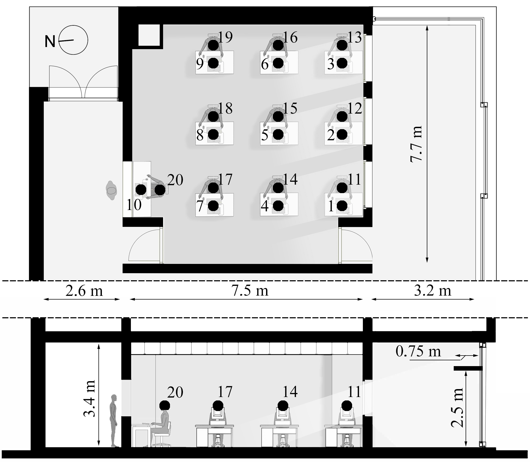
Fig. 1. Plan and section of the office.

The considered office consists in a South exposed almost squared room at the ground plane (7.5 m × 7.7 m) with three windows (1.5 m × 1.5 m) and a glass door (1 m × 2.2 m). The windows do not look directly on the outside, but on a greenhouse 3.2 m deep. There are 9 workspaces in the office with the desk disposed, as showed in Fig. 1. A tenth desk is located at the bottom of the room, in front of the north wall since it constitutes an information desk.

The dynamic simulation was carried out for 20 calculation points: 10 located at the height of the workplane (0.75 m from the floor) each one at the center of a desk and 10 placed at the eye-level of each user located on vertical planes (1.2 m from the floor). Since the room is used as an office where workspaces are equipped with computers, the medium maintained illuminance indicated by the standard is 500 lx [27]. Furthermore, the simulation was only performed for the working hours, hypothesizing that the office will be used from Monday to Friday from 9:00 to 18:00 (eight working hours plus one hour of lunch break) and that they will be closed on Saturday, Sunday and on holidays. The simulation time-step is equal to one hour. The referential weather database is the IWEC file referred to the city of Naples and freely available on the U.S. Departement of Energy website [28]. For the calculation of daylight related illuminance, the software Autodesk 3ds Max Design^® 2013 was used. The majority of the materials in the scene were modeled as diffusing, except for aluminum and stone, for which a specular reflection component was considered respectively equal to l7% and 15%.

Table 1 lists calculation parameters related to the materials modeled in 3ds Max Design^®, while rendering parameters related to the calculation or direct and indirect light are reported in Table 2.

Table 1

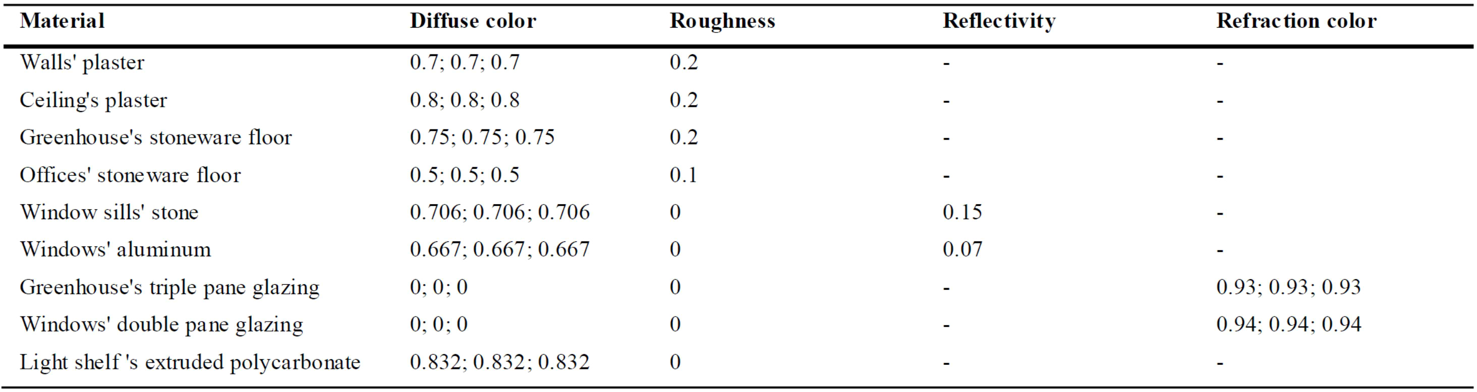
Table 1. Calculation parameters related to the materials modeled in 3ds Max Design^®.

Table 2

Table 2. 3ds Max Design^® rendering parameters [15].

3ds Max Design^® does not provide specific features to evaluate impact of shading devices or to compare different control systems. For this reason, the following methodology is proposed.

As regards shading devices design, two different simulations were performed. The former one considered that the greenhouse external facade was equipped with a system of light shelves 0.75 m deep and located at a height of 2.5 m from the floor (see Fig. 1). The second one was related to a simple fenestration system without light shelves. An analysis of the incidence of direct sunlight was performed. Considering that results demonstrated that light shelves reduce disability glare discomfort but not completely eliminate it, the critical hours for which discomfort risks probability are higher were computed. For these hours, the use of simple venetian blinds was simulated, and the results of the two simulations (only light shelves and light shelves plus venetian blinds) were integrated. UDI values were then calculated.

Finally, considerations about the possible configurations of an open-loop daylight-linked control system based on an external photosensor placed on the building's roof were presented.

In offices' applications the use of daylight-linked control can determine energy savings comprised between 20% and 31%, depending on the geographical location (latitude and longitude), the building's architectural configuration and the facade typology (type of window and of shadings) [29].

To model the functioning of such a system is very complex because its performances are affected by many factors: the photosensor's typology, its characteristics (spatial and spectral response), its location, the ratio between photosensor signal and workplane illuminance, and the adopted control strategy [29,30]. Not all these factors can be considered during calculation process, and also the most sophisticated software neglect some of these aspects.

For this particular application, the control system was simulated as following. Photosensor is modeled as an external illuminance calculation point located on the roof. The relationship between photosensor illuminance and work-plane illuminance was analyzed during the entire year and the most representative value assumed by the ratio between them was selected in order to simulate the second point of the calibration procedure of a dimming open-loop control algorithm. The performances of three different control systems were compared: an ideal control for which each workspace is lit by a single independent luminaire that emits a different luminous flux depending on the photosensor signal; a control for which each row of luminaires is independent and all the luminaires belonging to the same row emit the same luminous flux; a control for which all the luminaires emit the same luminous flux depending on the photosensor signal.

Once established the control algorithm, it was possible to simulate system's functioning for the three different strategies and to compare their performances.

The performances evaluation was divided in the following phases:

for each simulated hour and each sensor point, starting from the daylight illuminance, the ideal electric light requirement in terms of illuminance was calculated. For example, if a sensor registered a daylight illuminance of 300 lx the electric light requirement was 200 lx (equal to the difference between the task illuminance and the daylight illuminance);
the annual electric light requirement was obtained as the sum of all hourly values calculated during the year and referred to each sensor (expressed in klx•h);
an ideal electric lighting system constituted by three rows of luminaires parallel to the window wall was hypothesized;
the annual electric light requirements related to the three different control strategies were calculated and compared with the ideal requirement computed in phase b).

The goal of this analysis is to underline the capability of exploiting daylight characteristics of each different control strategy independently from the corresponding energy savings.

For this reason, the characteristics of the lighting system and of the luminaires are not reported and the electric light requirements of the three different controls are expressed only in terms of illuminance (klx•h) and not in terms of energy costs (kWh).

3. Results

As previously mentioned, two different simulations were performed, one considering the impact of light shelves and the other considering a simple fenestration system. An analysis of discomfort risks was performed. The annual percentage for which sunlight incidence was registered on the workplane or at the eye-level was calculated, as shown in Fig. 2. The winter months (in particular January and December) present the highest risks of discomfort, due to the sunlight beams tilt angle. As showed in the graphs, light shelves allow to reduce these risks but do not completely eliminate them.

Figure 2

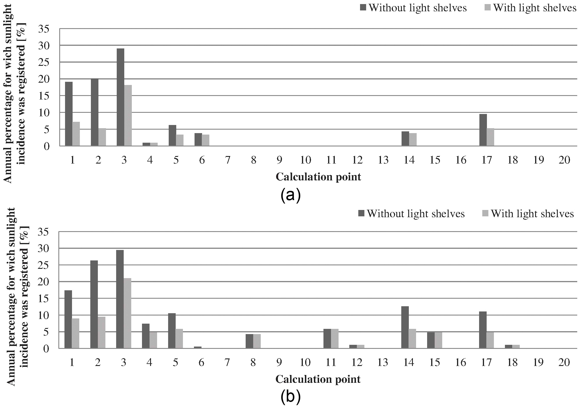
Fig. 2. Sunlight incidence on the workplane or at the eye-level for (a) January and (b) December.

The risk of discomfort occurs only during winter and in the first hours of the morning or in the evening, when solar rays are lower and the light shelves are not able to block them. Hypothesizing to shade each window with common venetian blinds, knowing the hours during which this phenomenon is verified, it was possible to understand for each time interval which shading has to be activated and which not. For example, if light comes from East, to block solar radiation, it is not necessary to close all the venetian blinds, but only the one located next to the workplace number 3 and the central one. If instead light comes from West only the venetian blind located next to workplace number 1 and the central one could be closed.

All the possible useful configurations were achieved by verifying all the occupied hours. The results related to January are reported in Table 3. In the first column, critical hours for which sunlight incidence is registered on the workplane or at the eye-level are reported. The other columns specify if each of the three venetian blinds must be closed or not in order to avoid discomfort.

Table 3

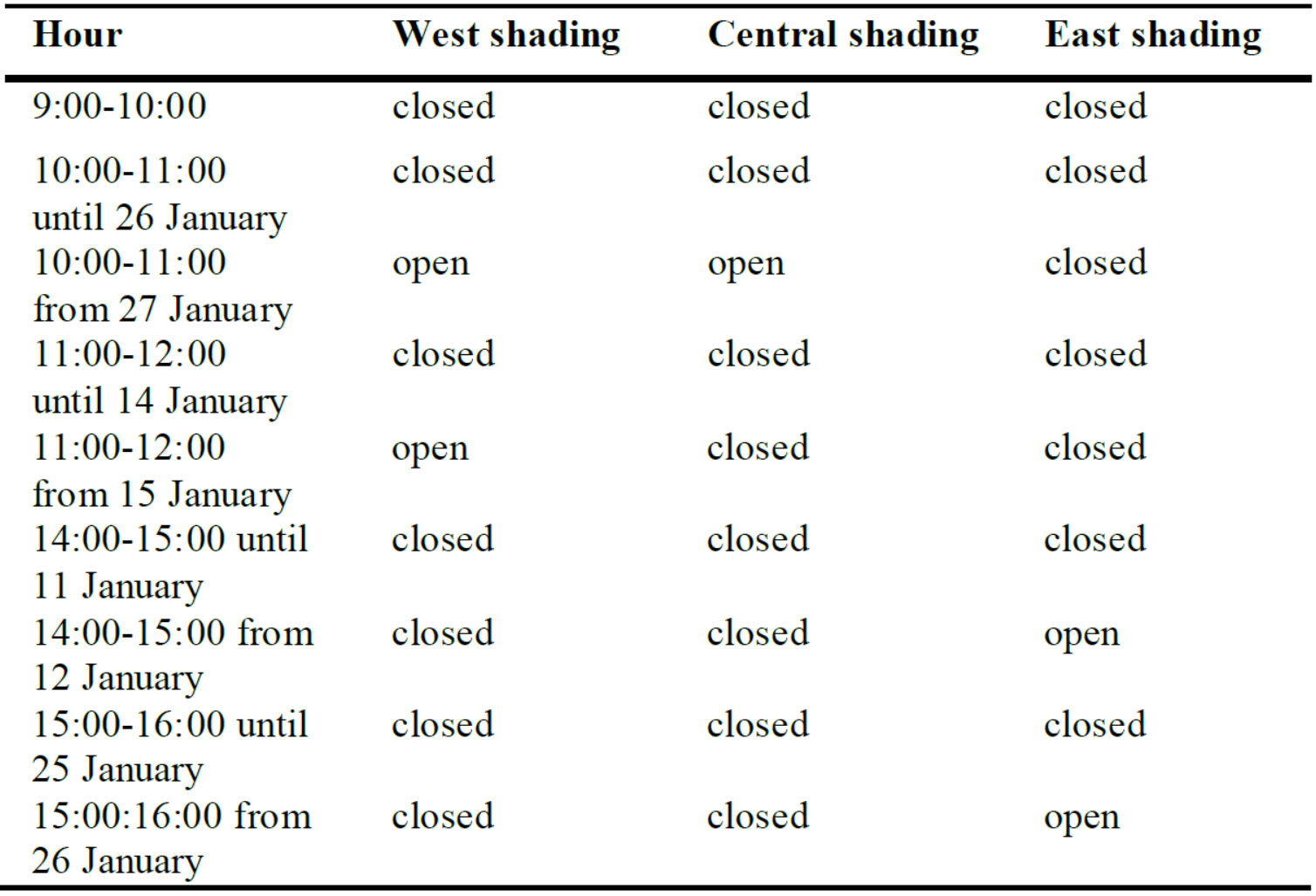
Table 3. Shadings configuration during January.

Taking into account the obtained results, a second simulation related to the hours during which it was necessary to use a shading system was carried out.

Integrating the results of the first and second simulations, daylight related illuminance levels were calculated. They were referred to an ideally comfortable and energy efficient situation, for which the shading system is only active when it is necessary to avoid glare while they are always open in the other cases. In this way daylight entrance is maximized. These light levels could be achieved only using an automated shading control system. Unfortunately, for manually activated shadings, 3ds Max Design^® does not include the possibility to calculate the variation in illuminance values, caused by the different users' behavioral patterns.

UDI values referred to the calculation points placed on the workplane were calculated basing on this ideal condition and are reported in Table 4.

Table 4

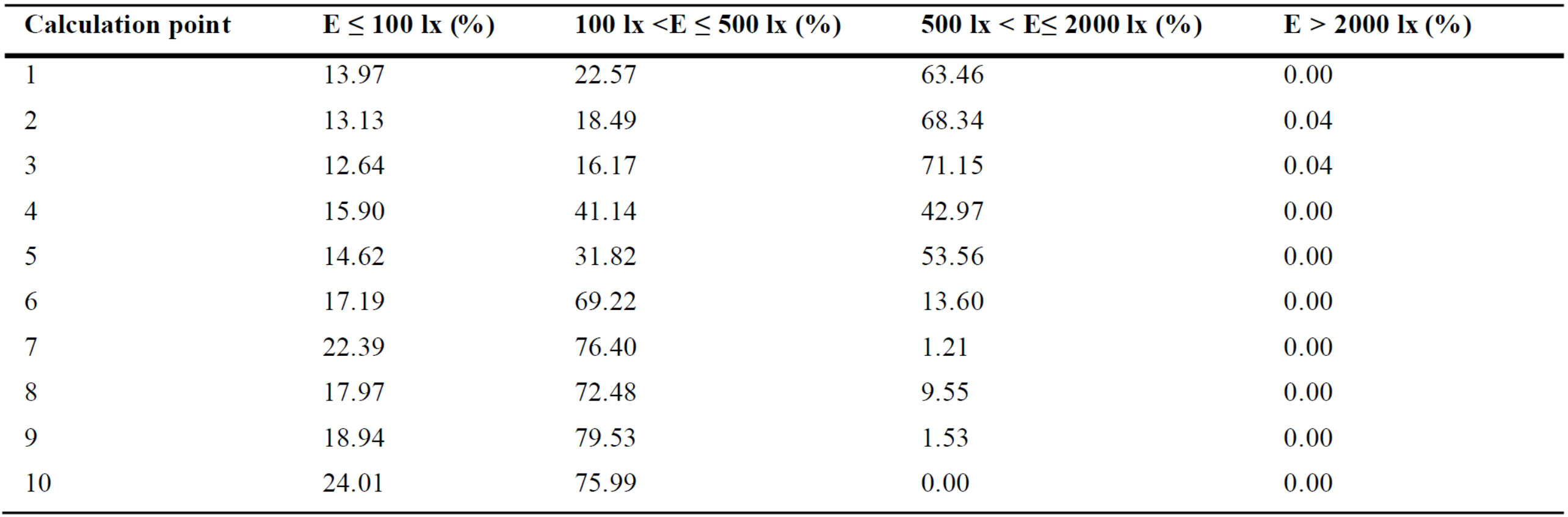
Table 4. UDI values related to the calculation points on the workplane.

From the table it is clear that daylight related levels can be considered as optimal for sensors corresponding to the first row of desks. Indeed for these points, for over 60% of the year daylight alone is able to lit the workplane, whereas for sensors like number 10 it is always necessary to use electric light.

The second part of the analysis was about the comparison of the three different control strategies described in Method section.

The first part of this analysis consists in calculate the ideal annual electric light requirement in terms of workplane illuminance for each workplace and defined considering only the daylight availability. Table 5 reported related results computed as defined in Method section at the point a) and b).

Table 5

Table 5. Ideal annual electric light requirement for each workspace.

Obviously requirements are different depending on the distance of the workplace from the window but some differences are observed also for sensors belonging to the same row.

Graphs reported in Fig. 3 show the correlation between the photosensor and the workplane daylight illuminances, together with the trend line characteristic of each sensor.

Figure 3

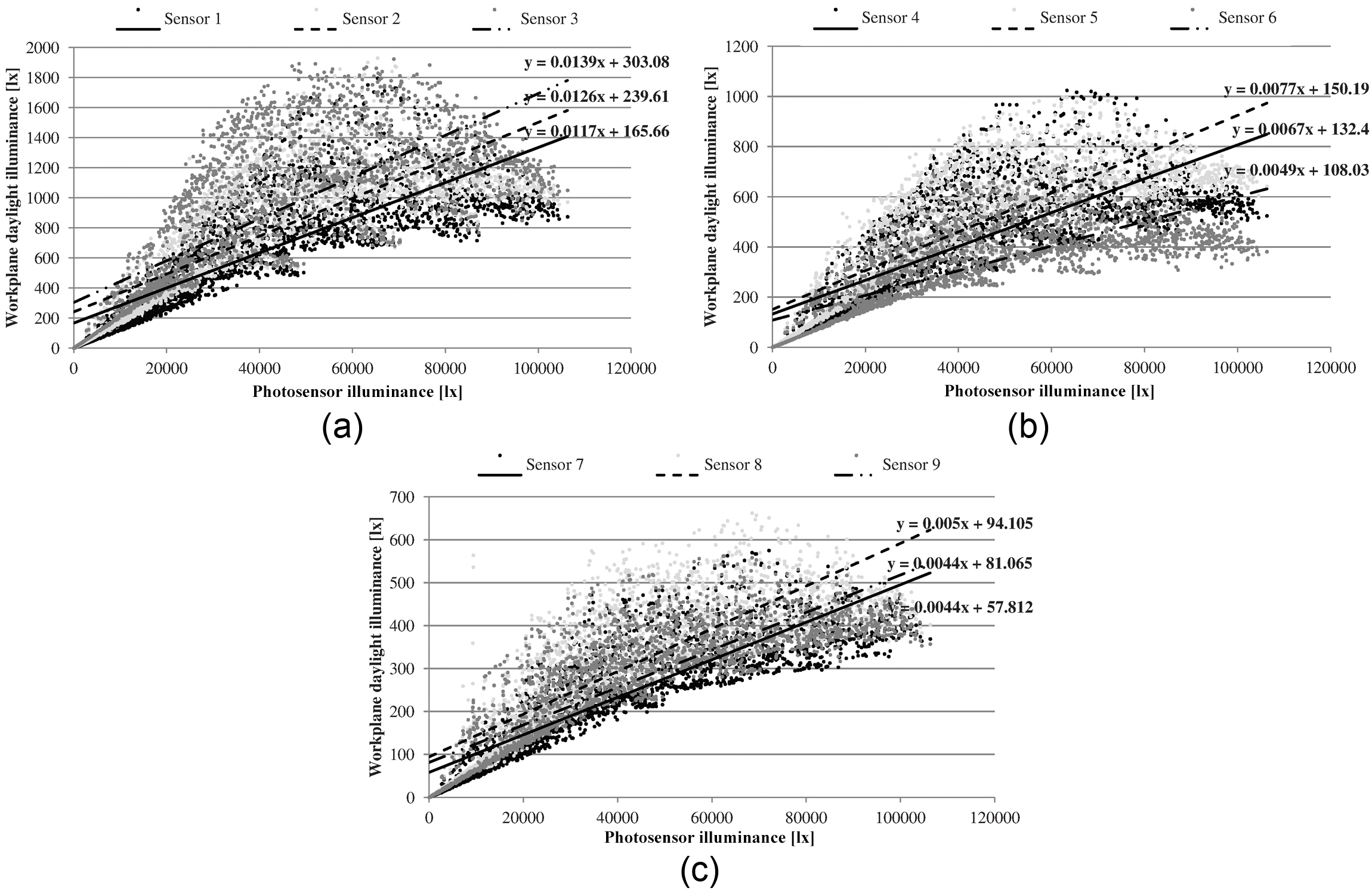
Fig. 3. The correlation between photosensor signal and workplane daylight illuminance for (a) first, (b) second, and (c) third row of sensors.

In a daylight-linked control this correlation is fundamental and it is the basis of the calibration process of the system [30]. In particular for an open-loop dimming control the calibration "consists of establishing the relationship between the photosensor reading and the daylight delivered to a critical location on the task plane at a representative daylight condition (which is present at calibration time). The calibration setting determines the linear relationship between the photosensor signal and the desired dimming level that is applied under all other daylight conditions" [30]

The photosensor signal does not necessary correspond with photosensor illuminance “because the photocell has its particular spectral and spatial response, which often does not match that of an illuminance meter” [31]. Considering that the dynamic daylight simulation software does not allow to model sensor characteristics and then to simulate its signal, the analysis of the ratio between daylight on the workplane and that sensed by the photocell can be based only on the photosensor illuminance.

The control algorithm needs two points in order to be defined: the first one corresponds to a nighttime signal of zero and the second one to a particular field measurement. In Fig. 3, the second point necessary for calibration can be identified. Through the trend lines, it is possible to establish that what is the most representative value of the ratio between photosensor signal and workplane illuminance. For example, considering the first row of sensors, an external illuminance of 20000 lx can well represent an indoor condition characterized by an illuminance of 400 lx at the Sensor 1.

In this way, it was possible to simulate a calibration process and to deduce the corresponding control algorithms as reported in Fig. 4.

Figure 4

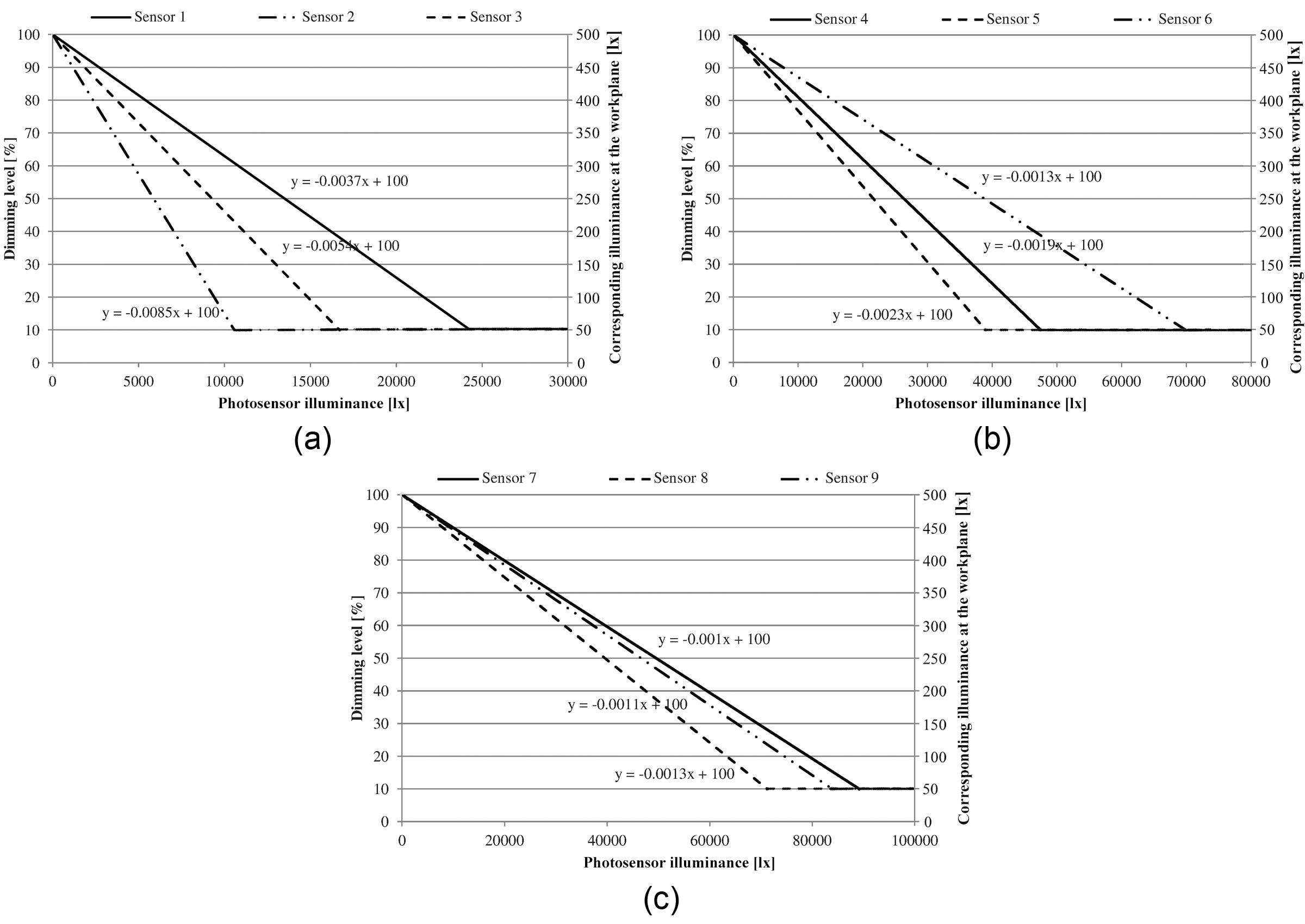
Fig. 4. Open-loop dimming control algorithm for (a) first, (b) second, and (c) third row of sensors.

The control algorithm is defined for each sensor of the analysis grid. In this way, it is possible to calculate the electric light requirements referred to the three control systems indicated at point d). For the first system, it was supposed that each workplace is lit by a different luminaire controlled through the corresponding algorithm reported in the graphs. In the second case, each row of luminaires is controlled by the algorithm corresponding to the most disadvantaged sensor of the row. In the third case, all the luminaires are controlled through the algorithm corresponding to the most disadvantaged sensor of the office.

Tables 6 and 7 reported the electric light requirements referred to the three control systems and their ratio with the requirements reported in Table 5 and calculated with the daylight simulation.

Table 6

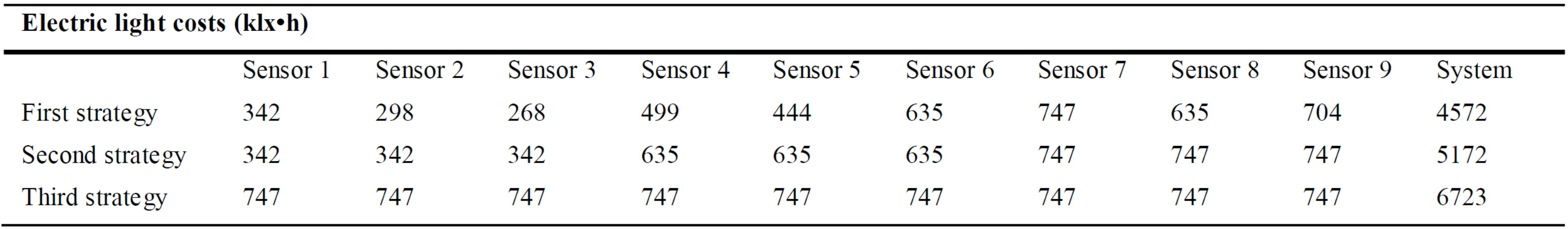
Table 6. Electric light costs related to the different control strategies.

Table 7

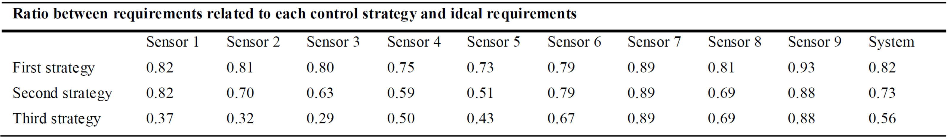
Table 7. Ratio between requirements related to each control strategy and ideal requirements calculated by simulation.

As it was easy to predict, the first ideal strategy is the most efficient whereas the third is the worst one, but it represents a typical control configuration considering standard applications. The low ratio referred to the third system is due to the difficulty to correlate the external daylight conditions to the indoor daylight distribution. As demonstrated by the graphs in Fig. 3, for a specific external illuminance value, there is a wide range of corresponding internal illuminances and vice versa; moreover, each point of the workplane can be characterized by a different curve that correlates indoor and outdoor conditions. When all luminaires are controlled through the same algorithm, the point chosen for the calibration is the most disadvantaged. This leads to the necessity for the system to emit a higher luminous flux with corresponding higher costs.

4. Discussion and conclusions

The paper has presented results related to a dynamic daylight simulation, which is carried out for an open-plan office and performed with 3ds Max Design^®. It proves that this software can be very useful in daylighting design applications, despite its use is not very widespread for this purpose. Furthermore, it allows to exploit the same geometric model, which is used for architectural design purposes, also for lighting analysis and to perform simulations in the same workspace used to produce photorenderings. This can simplify calculation procedures.

The software can be useful to design shading systems, evaluate the effect of these systems on indoor daylight availability, or compare the performances of different lighting controls more or less complex. It is also clear that simulation results are based on an ideal model, which does not perfectly correspond to reality. For example, as regards this particular application, shading devices are modeled as an ideal system, which does not consider users' behavior. Software like Daysim or DIVA [32,33] present internal calculation models that allow to ride out this inconvenience [9]. There are problems also with control systems' modeling. For example, the calculation of the lighting requirements is reported only in terms of light requirements and not in terms of energy consumptions. Some software [32,33] allow to predict energy costs but their evaluations are still vague. In [34], they demonstrated that evaluating energy costs with different software can determine results that diverge up to 15%. On the one hand differences in results depend on the definition of indoor daylight availability, but on the other hand they depend on the control systems' modeling that neglect important factors as the specific characteristics of photosensors, luminaires, or ballasts [20–23].

Even though these calculation techniques are very useful in the entire design process, experimentations are necessary to improve software performance in order to make calculation models more similar to realistic conditions.

Contributions

L. Bellia conceived the study. F. Fragliasso performed the dynamic daylight simulation, processed results, and wrote the manuscript with input from all the authors. A. Pedace contributed to the results analysis. All the authors discussed the results.

References

J. Mardaljevic, Simulation of annual daylighting profiles for internal illuminance, Lighting Research and Technology 32 (2000) 111–118. http://dx.doi.org/10.1177/096032710003200302
J. Mardaljevic, C. Reinhart, and Z. Rogers, Dynamic daylight performance metrics for sustainable building design, Leukos 3 (2006) 7–31. http://dx.doi.org/10.1582/LEUKOS.2006.03.01.001
J. Love and M. Navvab, The vertical-to-horizontal illuminance ratio: A new indicator of daylighting performance, Journal of the Illuminating Engineering Society 23 (1994) 50–61. http://dx.doi.org/10.1080/00994480.1994.10748080
J. Mardaljevic, Simulation of annual daylighting profiles for internal illuminance, Lighting Research and Technology 32 (2000) 111–118. http://dx.doi.org/10.1177/096032710003200302
CIE Technical Report Daylight, CIE, Vienna, 1970.
C. F. Reinhart and O. Walkenhorst, Validation of dynamic RADIANCE-based daylight simulations for a test office with external blinds, Energy & Buildings 33 (2001) 683–697. http://dx.doi.org/10.1016/S0378-7788(01)00058-5
Z. Rogers, Daylighting Metric Development Using Daylight Autonomy Calculations In the Sensor Placement Optimization Tool, 2006, Available at: http://www.archenergy.com/SPOT/download.html.
A. Nabil and J. Mardaljevic, Useful daylight illuminance: a new paradigm for assessing daylight in buildings, Lighting Research and Technology 37 (2005) 41–57. http://dx.doi.org/10.1191/1365782805li128oa
C. Reinhart, Tutorial on the Use of Daysim Simulations for Sustainable Design, 2006, Available at: http://archive.nrc-cnrc.gc.ca/obj/irc/doc/daysim-tutorial.
C. E. Ochoa, M. B. C. Aries, and J. L. M. Hensen, State of the art in lighting simulation for building science: a literature review, Journal of Building Performance Simulation 5 (2012) 209–233. http://dx.doi.org/10.1080/19401493.2011.558211
J. Mardaljevic, Validation of a lighting simulation program under real sky conditions, Lighting Research and Technology 27 (1995) 181–188. http://dx.doi.org/10.1016/j.solener.2012.11.020
J. Mardaljevic, The BRE-IDMP dataset: a new benchmark for the validation of illuminance prediction techniques, Lighting Research and Technology 33 (2001) 117–134. http://dx.doi.org/10.1177/136578280103300209
C. F. Reinhart and S. Herkel, The simulation of annual daylight illuminance distributions — a state-of-the-art comparison of six RADIANCE-based methods, Energy and Buildings 32 (2000) 167–187. http://dx.doi.org/10.1016/S0378-7788(00)00042-6
A. A. Freewan, Maximizing the Performance of Laser Cut Panel by Interaction of Ceiling Geometries and Different Aspect Ratio, Journal of Daylighting 1 (2014) 29–35. http://dx.doi.org/10.15627/jd.2014.4
C. Reinhart and P.-F. Breton, Experimental Validation of 3ds Max Design 2009 and Daysim 3.0, in: Proceeding of the 11th International IBPSA Conference, 2009, Glasgow, Scotland.
R. Perez, R. Seals, and J. Michalsky, All-weather model for sky luminance distribution—Preliminary configuration and validation, Solar Energy 50 (1993) 235–245. http://dx.doi.org/10.1016/0038-092X(93)90017-I
A. Iversen, S. Svendsen, and T. R. Nielsen, The effect of different weather data sets and their resolution on climate-based daylight modelling, Lighting Research and Technology 45 (2012) 305–316. http://dx.doi.org/10.1177/1477153512440545
L. Bellia, A. Pedace, and F. Fragliasso, The role of weather data files in Climate-based Daylight Modeling, Solar Energy 112 (2015) 169–182. http://dx.doi.org/10.1016/j.solener.2014.11.033
C. F. Reinhart, Lightswitch-2002: a model for manual and automated control of electric lighting and blinds, Solar Energy 77 (2004) 15–28. http://dx.doi.org/10.1016/j.solener.2004.04.003
A. Choi, K. Song, and Y. Kim, The characteristics of photosensors and electronic dimming ballasts in daylight responsive dimming systems, Building and Environment 40 (2005) 39–50. http://dx.doi.org/10.1016/j.buildenv.2004.07.014
L. Doulos, A. Tsangrassoulis, and F.V. Topalis, The role of spectral response of photosensors in daylight responsive systems, Energy and Buildings 40 (2008) 588–599. http://dx.doi.org/10.1016/j.enbuild.2007.04.010
L. Doulos, A. Tsangrassoulis, and F. Topalis, Quantifying energy savings in daylight responsive systems: The role of dimming electronic ballasts, Energy and Buildings 40 (2008) 36–50. http://dx.doi.org/10.1016/j.enbuild.2007.01.019
C. Ehrlich and K. Papamichael, Judy Lai, Kenneth Revzan, A method for simulating the performance of photosensor-based lighting controls, Energy and Buildings 34 (2002) 883–889. http://dx.doi.org/10.1016/S0378-7788(02)00064-6
IES-LM-83-12, Approved Method: IES Spatial Daylight Autonomy (sDA) and Annual Sunlight Exposure (ASE), 2013.
USGBC, LEED Reference Guide for Building Design and Construction (v4). US Green Building Council, 2014, Available at: http://www.usgbc.org/resources/leed-reference-guide-building-design-and-construction.
Satel-light, Available at: http://www.satel-light.com.
UNI EN 12464-1:2011 - Light and lighting - Lighting of work places - Part 1: Indoor work places.
Weather data, U.S. Departement of Energy, Available at: http://apps1.eere.energy.gov/buildings/energyplus/weatherdata_about.cfm?CFID=1273318&CFTOKEN=3cea6aeda668df5d-6CC0143E-E638-ACEA-CCF5C27742B7095E .
M. Asif ul Haq, M. Yusri Hassan, H. Abdullah, H. Abdul Rahman, M. Pauzi Abdullah, F. Hussin, and D. Mat Said, A review on lighting control technologies in commercial buildings, their performance and affecting factors, Renewable and Sustainable Energy Reviews 33 (2014) 268–279. http://dx.doi.org/10.1016/j.rser.2014.01.090
D. L. Di Laura, K. W. Houser, and R. G. Mistrick, Lighting controls, Lighting Handbook, 10th Edition, Illuminating Engineering Society, 2011.
NLPIP National Lighting Product Information Photosensors Program - Dimming and Switching Systems for Daylight Harvesting, 2007.
Daysim, Available at: http://daysim.ning.com.
DIVA, Available at: http://diva4rhino.com.
L. Doulos, A. Tsangrassoulis, and F. V. Topalis, A critical review of simulation techniques for daylight responsive systems, in: Proceedings of the European Conference on Dynamic Analysis, Simulation and Testing applied to the Energy and Environmental performance of buildings, 2005, Athens, Greece.

Get PDF (2.79 MB)

SHARE ON