Lighting Energy Saving with Light Pipe in Farm Animal Production

^a Swedish University of Agricultural Sciences, Department of Biosystems and Technology, Box 103, SE-23053 Alnarp, Sweden.
^bLund University, Institute for Architecture and the Built Environment, Division of Energy and Building Design, Box 118, 221 00 Lund, Sweden.

* Corresponding author. Tel: +46 40 41 54 85
hans.von.wachenfelt@slu.se (H. v. Wachenfelt)
vaia.vakouli.379@student.lu.se (V. Vakouli)
alejandro.pacheco@bau.se (A. P. Diéguez’)
niko.gentile@ebd.lth.se (N. Gentile)
marie-claude.dubois@ebd.lth.se (M.-C. Dubois)
knut-hakan.jeppsson@slu.se (K.-H. Jeppsson)

History: Received 29 June 2015 | Revised 1 September 2015 | Accepted 2 September 2015 | Published online 8 September 2015

Citation: Hans von Wachenfelt, Vaia Vakouli, Alejandro Pacheco Diéguez’, Niko Gentile, Marie-Claude Dubois, and Knut-Håkan Jeppsson, Lighting Energy Saving with Light Pipe in Farm Animal Production, Journal of Daylighting 2 (2015) 21-31. http://dx.doi.org/10.15627/jd.2015.5

Figures and tables

Figure 1
Figure 2
Figure 3
Figure 4
Table 1
Figure 5
Figure 6
Table 2
Table 3
Figure 7
Figure 8
Figure 9
Figure 10
Figure 11
Figure 12
Figure 13
Table 4
Figure 14
Figure 15

Abstract

The Swedish animal production sector has potential for saving electric lighting of €4-9 million per year using efficient daylight utilisation. To demonstrate this, two light pipe systems, Velux^® (house 1) and Solatube^® (house 2), are installed in two identical pig houses to determine if the required light intensity, daylight autonomy (DA), and reduced electricity use for illumination can be achieved. In each house, three light sensors continuously measure the indoor daylight relative to an outdoor sensor. If the horizontal illuminance at pig height decreases below 40 lux between 08.00 and 16.00 hours, an automatic control system activates the lights, and electricity use is measured.. The daylight factor (DF) and DA are determined for each house, based on annual climate data. The mean annual DA of 48% and 55% is achieved for house 1 and house 2, respectively. Light pipes in house 2 have delivered significantly more DA than those in house 1. The most common illuminance range between 0 and 160 lux is recorded in both houses, corresponding to approximately 82% and 83% of daylight time for house 1 and house 2, respectively. Further, the daylighting system for house 2 has produced a uniform DF distribution between 0.05 and 0.59. The results demonstrate that considerable electric energy savings can be achieved in the animal production sector using light pipes. Saving 50% of electric lighting would correspond to 36 GWh or 2520 t CO₂ per year for Sweden, but currently the energy savings are not making the investment profitable.

Keywords

Light pipe; Daylighting; Energy saving; Electric lighting

1. Introduction

Electric lighting is directly responsible for 19% of the world’s electricity consumption [1]. Light pipes offer a passive way to bring daylight to rear spaces in deep buildings, such as animal houses. In Sweden, the Swedish Board of Agriculture [2] and European regulations [3] regulate daylight and electric lighting intensity in pig houses. This study assesses the energy saving potential of two commercial light pipe systems by measuring illuminance in two existing full-scale pig houses located near Lund, Sweden.

Almost one-fifth of the electricity produced globally is consumed by the lighting sector. The total annual cost of electric lighting in 2006 represented about 1% of the global GDP, i.e. USD 360 billion, and electricity use being directly responsible for two thirds of that value [1]. The Swedish animal production sector has potential for electric lighting savings in the range of €4-9 million per year through improved daylight utilisation [4,5], based on an electricity price of €0,11 per year.

Daylighting is one of the most obvious ways to reduce electric lighting consumption. The greatest challenge for daylighting systems is to deliver the light deep within buildings. Daylight utilisation has also proven to increase resident sociability, well-being, productivity, and health in humans [6–8]. Daylight also improves mood and vigilance in humans because it is directly linked to the circadian cycle, and it has similar effects for many animal species [9].

The minimum illuminance for pigs is 40 lux for a minimum period of 8 hours per day, as stated in European legislation [3]. Pig houses should have windows or other daylight inlets according to Swedish Board of Agriculture regulations [2]. Large low-buildings dominate the animal production sector, and windows present in these buildings give a poor core daylighting effect. Compact insulated buildings are necessary for growing animals, such as pigs, and poultry and light pipe technology can be an effective way to provide daylight in such compact buildings.

The light levels in pig pens should permit pig communication and identification of pen features, such as feeders. The EU recommended illuminance of 40 lux has not been shown to be either disliked or strongly preferred by pigs [10]. There is good evidence that pigs' eyes are not adapted for extremely bright light [11], and they may prefer dim natural light levels [12]. Pigs prefer to sleep in dim lighting/darkness (2.4 lux), suggesting that lying areas of the pen should not be brightly lit in order to promote resting behaviour [11]. The increased photoperiod increases food intake in growing pigs [13,14]. A key benefit of natural lighting is that it provides dawn and dusk periods, reducing the competition for feed when lights are switched on in the morning and reducing potentially startling effects when lights are switched on or off.

Light pipes can bring daylight to deep interior spaces and provide a natural spectrum and dynamic variations that are typical in nature. Light pipes present the advantage of effectively capturing direct beam radiation from the sun while avoiding excessive heat gains and glare patches. The main drawback is that their performance is greatly affected by sky clearness, as they produce much lower light levels under overcast sky conditions [15,16]. Light pipes are thus better suited for climates with predominantly clear skies [17], while the climate in Sweden gives a very high proportion of overcast skies. The proportion of direct/diffuse radiation in Sweden is only about 1/1 [18], which is quite low compared to most countries. However, since the light levels preferred by animals, such as pigs, are quite low, light pipes may still be suitable in this context.

One of the main light pipe manufacturer recommends that the space served by the light pipes should not exceed 9 meters from the rooftop in order to give acceptable light levels. Therefore, they are suitable for rooms on the top floor [19], large one-story buildings like industrial units, sheds, or livestock houses.

The overall aim of this study is to demonstrate the potential for a reduction of electricity use for lighting in farm buildings by analysing how much of the electrical energy could be replaced by daylight through light pipes and the effect on animal lighting environment. The specific objective is to determine the efficiency of light pipe daylight systems and their function in the daily operation of a pig house with a soiling environment. The hypothesis is that the daylighting systems give an acceptable uniform lighting environment with 40 lux in the animal living area for sufficiently many operating hours for the energy-saving to repay the investment.

The remainder of this paper is organised as follows. Section 2 describes the light pipe systems that are used for daylighting in two identical pig houses, the experimental design, and how the data is recorded and processed. The results are reported in Section 3. In Section 4, daylight autonomy (DA), recorded illuminance, daylight distribution, and daylight factor (DF) are discussed and compared with respect to the two systems, and a critical analysis of the data collection method used along with design considerations are presented. Finally, conclusions are presented in Section 5.

2. Materials and methods

The pig houses are located in Odarslöv (55°45'N, 13°15'E), Sweden. The skies at the site are predominant overcast in the winter and mixed in the rest of the year. Midday solar altitude ranges from 11º on December 21 to 58º on June 21.

2.1. Houses

Two full-scale, inhabited and identical pig houses, located next to each other, were fitted with four light pipes, each located in the same position in each house. The light pipes in house 1 (Velux Sun Tunnel^®) on the eastern side had a bend in connection with a flat collector, while the pipes in house 2 (Solatube Brighten Up^®), on the western side were straight and had a dome collector equipped with a reflector to redirect low-angle sunlight (Figs. 1 and 2). The light pipes were installed on a pitched roof with a 22º tilt angle, facing approximately north-south, and half the light pipes in each house were located on the southern pitch and the other half on the northern pitch.

Figure 1

Fig. 1. Cross-section A of house 1.

Figure 2

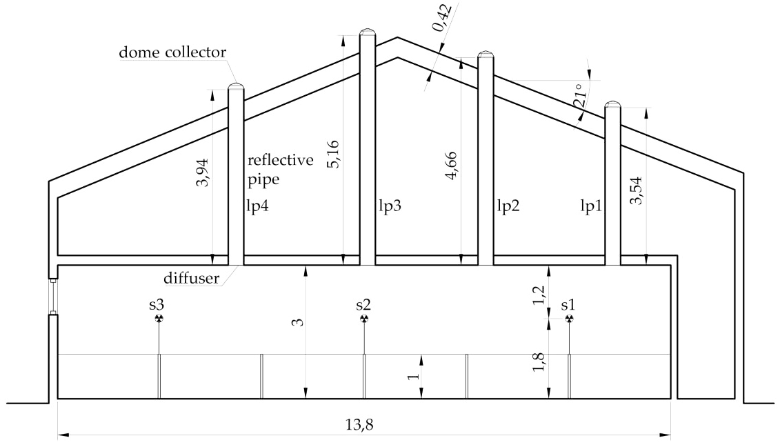
Fig. 2. Cross-section B of house 2.

The interior floor dimensions of the houses were approximately 13.8 m × 6.1 m with height of 3 m, as shown in Fig. 3. Each house had an inspection aisle with six pens along it, with 15 growing finishing pigs in each pen. All light pipes were installed following a center line along the pig pens, directly above the animal feeding troughs. The dunging area is located close to the inspection aisle, and the animal resting area is furthest away from the aisle, with an isolating and light shading cover on top of the pen dividing walls (Fig. 3). Apart from the light pipes, each stable had a window in the north wall to provide daylight in the interior.

Figure 3

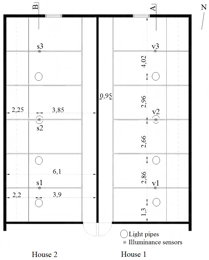
Fig. 3. Plan of houses 1 and 2 with cross-sections marked A and B, respectively.

2.2. The light pipe

The light pipes consisted of three components: a collector, a reflective pipe and a diffuser, as shown in Fig. 4. The optical properties of the both light pipes are listed in Table. 1. The collector was a transparent element, which was located at the external aperture of the pipe. Its main functions were to collect daylight and protect the light pipe from the impact of weather and soiling. It was usually made flat or dome-shaped from a highly transmitting material. In the present case, the light pipes that were used in house 1 had a flat collector consisting of a single-layer clear glass panel fastened at the light pipe’s upper aperture. Those used in house 2 had a dome collector consisting of a curved Fresnel lens that redirected sunlight from low solar altitudes into the pipe. This feature was proven to enhance the light efficiency of light pipes in the low sun conditions typical for high latitudes [20,21]. The dome collector of the light pipes, which was used in house 2, was also equipped with a light reflector, which could be classified as an optical redirecting system. It was a laser-cut panel, which was located within the dome collector and orientated towards the equator. Its purpose was to redirect low-angle incident beams of light into the pipe. Light penetration for low solar altitude angles (below 60º) was thus enhanced further by this technique [21,22].

Figure 4

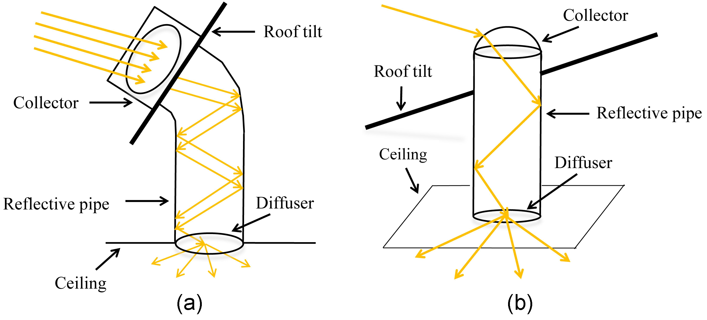
Fig. 4. Layout of the light pipe for (a) house 1 and (b) house 2.

Table 1

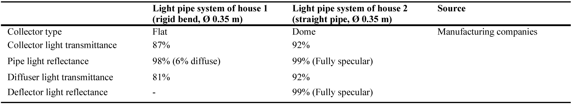
Table 1. Optical properties of the light pipe models.

The design of mirror light pipe (MLP) and optical properties are optimised for transmitting daylight from collector to diffuser with minimal light losses. Both light pipe models have circular cross-section (Fig. 4). The most important characteristic of the MLP design is its light reflectance, usually above 98%, but also the high specular reflectance for ultimate sunbeam function. The aspect ratio of the light pipe, i.e. the diameter to length ratio, determines the amount of light that bounces in the light pipe. The recommended aspect ratio is < 1/10, and it should never exceed 1/20, since longer light guides have very low light transmittance [16]. In this study, the aspect ratio of the two light pipe types ranged between 1/9 and 1/15 depending on the location of the pipes on the roof pitch and both models had a diameter of 0.350 m.

The light pipe diffuser was installed in the ceiling of the room, and usually took the form of an opal dome or a white flat polycarbonate disc. After solar altitude, the diffuser was the next most critical factor determining the light output distribution of light pipes [16]. In this study, the diffusers of the light pipes were flat and prismatic.

2.3. Electric lighting system

Each house had three ceiling-mounted 2×35 W T5 fluorescent tube fixtures (with plastic tube cover) that were connected to an electricity meter (Fig. 5). The fluorescent tubes were controlled by an automatic daylight on/off system (Turnus 771, Grässlin GmbH, Bundesstrase 36, 78112 St. Georgen, Germany), including a photosensor that produced signals to keep the lights on only when daylight was insufficient, i.e. below 40 lux [2,3]. Due to this low illuminance threshold, the location of the two photosensors inside the houses would have caused a continuous oscillation between on and off modes. To avoid this problem, the sensors were placed in the roof void, in an area shaded from sunlight. The threshold was then indirectly determined by calculating the illuminance ratio between the photodiode position and a representative point in the house. Based on the ratio, the threshold was set through the action of a small potentiometer. The time lapse for the sensor to change from on to off and vice versa was set to one minute.

Figure 5

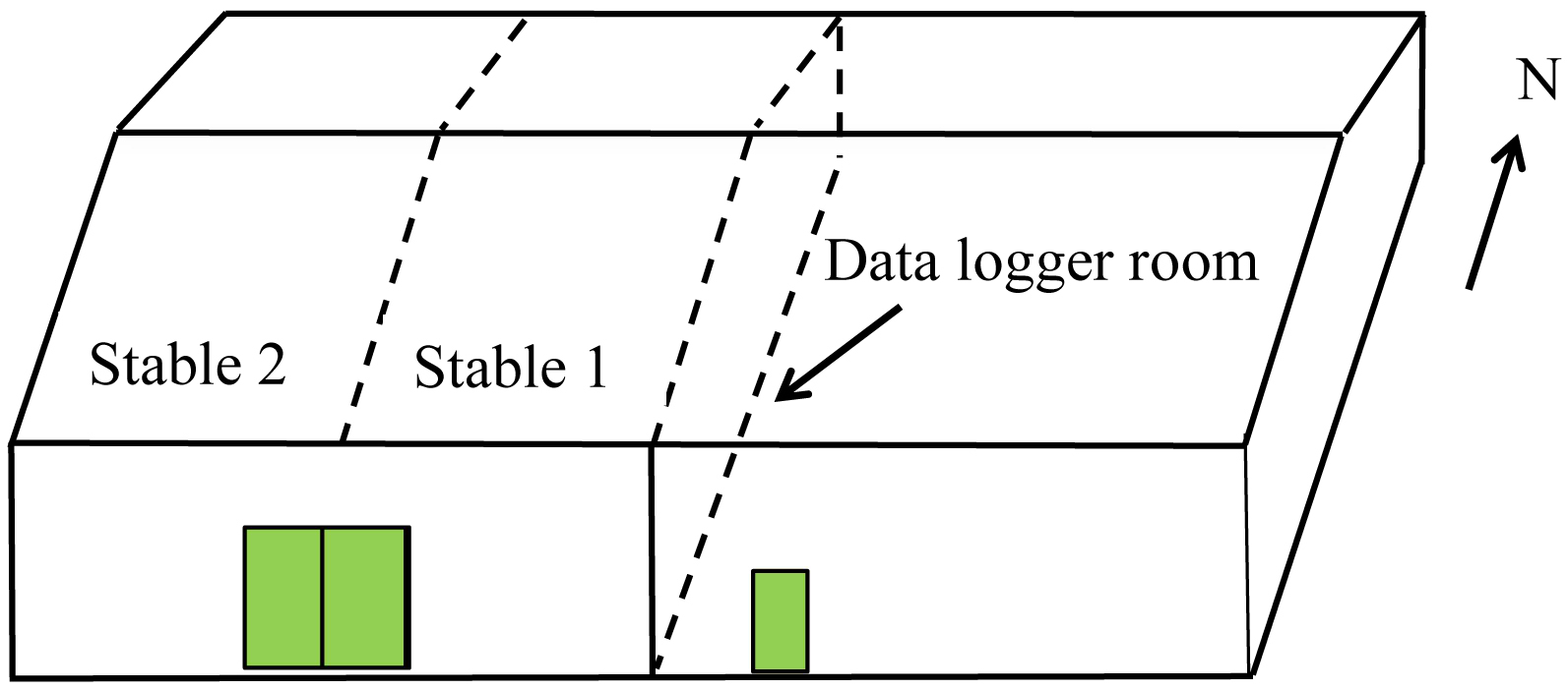
Fig. 5. Location of pig houses and data logger room in the building.

2.4. Measuring system

A system of illuminance sensors and electricity meters for the electric lights was installed to record the indoor and outdoor illuminance levels and the electricity consumption for the lighting system [23]. The data was collected by a logger, which was located in a service room adjoining the pig houses (Fig. 5). The daylight contribution of the north-facing windows to the sensors was not significant and was equal in both houses; therefore, it was not considered further.

The measuring system consisted of three indoor sensors for the interior horizontal illuminance in each house and one outdoor sensor for the global horizontal illuminance. The indoor illuminance meters (Hagner SD2 Light Sensor, B. Hagner AB, Sweden) were located in between the pig pens, along a dividing pen wall, at a height of 1.8 m above the floor along the centre line of the pig pens (Fig. 3), and they were set to measure the range between 0 and 2000 lux. The external illuminance meter (Hagner ELV-841 Light Sensor, B. Hagner AB, Sweden) was located in an unobstructed area near the building, and it was set to measure the range between 0 and 200000 lux. To protect them from the pig house environment, the sensors were fitted with waterproof cases and an electric heater to prevent moisture layers developing inside and on the cases. All sensors were calibrated by Hagner AB before delivery, and had a stated accuracy of ±3%. Both the indoor and outdoor illuminance meters generated a voltage as output to be sent to the data logger. The electricity consumption was measured by means of standard electricity meters, which generated a pulse signal as output (1000 pulses/kWh). The data logger (CR 1000, Campbell Scientific Inc. Logan, Utah, USA) acquired a signal from the light sensors every 10 seconds, and the signals were used to calculate a periodic average every six minutes and every hour.

2.5. Sensor soiling factor

The data received from the measuring system was reliable, but high variability was still found in the sensor data averaged every six minutes, especially with overcast skies. In practice, the measuring system collected variable values depending on the amount of soiling in the pig houses. A sensor soiling factor (SSF) was therefore determined to account for the accumulation of soiling on the sensors. Even when the sensors were regularly cleaned, the soiling accumulation was considerable. The sensors were cleaned on the evening of February 11, i.e. SSF = 0, which was detectable from sensor readings of the electric light illumination. This reading was the sole source of light, and the window was blacked out. For SSF calculation, the light conditions on February 12 at 09:18 AM were used as reference. This time was chosen for reference because it had light conditions that occurred every day, i.e. the electric lights were on, the daylight levels outdoors were low (i.e. global horizontal illuminance (GHI) = 8081 lux) and SSF = 0. A similar situation (lights on and about 8000 lux of GHI) was chosen for each of the days considered. For each of these days, the SSF was applied to each subsequent reading to correct for the soiling error. The SSF was calculated by

\[ SSF_{day-x} = \frac{E_{reference}}{E_{day-x}} \]

where SSF_day-x is the sensor soiling factor on a chosen day, E_reference is illuminance reading from the sensor at the reference moment (February 12 at 09:18; lights on and GHI = 8018 lux), and E_day-x is illuminance reading from the sensor on the chosen day at a moment when the electric lights were on and and the GHI was approximately 8000 lux.

2.6. Experimental design

Daylight and light values were collected continuously during the period September 2013 to December 2014. In November 2013, the outdoor sensor was failed and replaced by a new sensor on 17 December 2013. The data was imported and all calculations were performed using Microsoft Excel. The results were presented as periodic averages at every 6 minutes with time and date of recorded daylight, electricity consumption for each pig house, and GHI. During the measurement period, the DF was manually measured on two occasions.

2.7. Data recording and processing

From the continuous measurements of the light pipes, the calculated percentage of DA hours where the sensor illuminance was higher than 40 lux was determined during the year. In addition, the number of hours of electric lighting use and the energy saving potential due to DA with the light pipes were determined.

The calculations were carried out monthly for each pig house and lighting system. Using a conditional function, only daytime-recorded values, i.e. between 08.00 and 16.00 in winter and 07.00-15.00 in summer, were considered. If the electric lighting use was zero, the value was recorded in the DA calculation. To include the DA values that were omitted by the on/off sensor delay function, another condition was added. If the GHI value from the outdoor sensor was above 15 000 lux, the recorded value was classified as a potential DA value. To control the system, all recorded values per month and year were included.

The amount of sensor soiling was determined each day for the first three months of the year to calculate the SSF. The SSF mean and standard deviation (SD) based on single recorded values were 1.2 and 0.23, respectively, during these three months (n = 90). Internal reflection and soiling in the two houses (floor, walls, and ceiling) were assumed to be of the same order of magnitude, following regular cleaning intervals.

A mean value of illuminance at pig level was determined monthly for both the electric lighting and for daylight alone, and an illuminance frequency distribution was determined for each house. The calculation was performed by sorting the data from the original values using a conditional function and using only daytime recorded values. The calculation of electricity use and daylight was performed separately, but in the same way. The value was recorded as electric lighting, if the electricity use exceeded zero. The lighting value was valid at sensor height; therefore, to achieve a value at pig level, 0.7 m above floor level, the value was divided by a factor of 2.25, which was obtained by the illuminance ratio between sensor s1 and v1 position (450 lux) and illuminance at pig height (200 lux). The ratio was assumed constant. The SSF was applied to the measured value by multiplying the value by the average soiling factor of 1.2.

Manual measurement of the DF was carried out in June and November 2013 without pigs [24]. The reference points were determined on a 9-point grid at 0 m and 1.5 m above the floor. Daylight reached the grid points from the light pipes and from a window in the far end of each house. The distance from the measuring point to the nearest light pipe was calculated using information in Figs. 1–3.

2.8. Statistical analyses

A paired t-test was performed to determine whether there was a difference in daylight collection and monthly DA between the two light pipe systems. The data was tested for normal distribution, and the level of statistical significance was set to p < 0.05 throughout the analysis, which was performed in Minitab™ [25]. An analysis of variance, PROC MIXED in SAS Institute Incorp. [26], was performed for each measuring height in the houses to determine the effect of DF depending on grid measuring point in the house and light pipe system. The statistical model was a split-plot design with measuring occasion as a block effect, house as main effect, and measuring point as split-plot effect. A significance level of p < 0.05 was used throughout the analysis, and Tukey’s method was used to separate treatment means. The statistical model is by

\[ Y_{ijk} = μ + a_i + b_j + \delta_{ij} + γ_k + {aγ}_{ik} + ε_{ijk} \]

where μ is the treatment mean, α_i is the stable, b_j is the random effect of measuring occasion, γ_k is the measuring point, ε_ijk is the error term, i is the stable (1, 2), j is the measuring occasion (1, 2, …, 8), and k is the measuring point (1, 2, …, 9).

3. Results

3.1. Daylight autonomy

The DA recordings at sensor level were typically 7439 per month and 6719 in February. The illumination by daylight was generally low under 10% during January, but increased rapidly during the following months. In March, DA provided more than 50% of the total illumination hours in both light pipe systems. The mean total annual DA, or energy saving, was 48% for house 1 and 55% for house 2, with a mean DA of approximatly 51% and 57% in the first half year and 45% and 52% in the second half year for house 1 and house 2, respectively (Fig. 6). Total DA and use of electricity for lighting is shown in Table 2. At present, a light pipe investment of 20 light pipes with a total price of €15800 in a pig house, using 9000 kWh per year based on 50% energy saving, a 10 year economic payback period and 3% interest rate, reveal a need for an electricity cost of €0.47 per kWh for the producer to make the investment profitable. Pair-wise comparison of DA percentage during the year showed that the light pipe system in house 2 delivered significantly more DA than the system in house 1 (Table 3). All data followed a normal distribution.

Figure 6

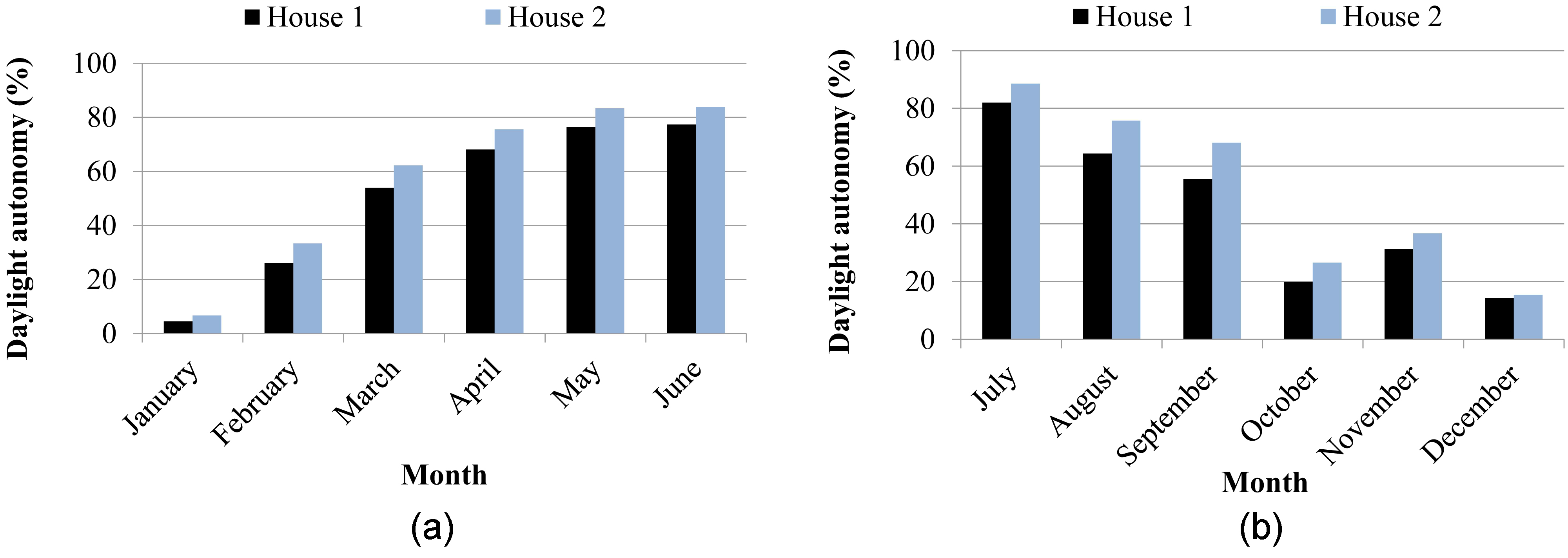
Daylight autonomy at sensor level, based on measurements from (a) January-June and (b) July-December of two light pipe systems installed in two pig houses at Odarslöv (55°45'N, 13°15'E), Sweden.

Fig. 6. Daylight autonomy at sensor level, based on measurements from (a) January-June and (b) July-December of two light pipe systems installed in two pig houses at Odarslöv (55°45'N, 13°15'E), Sweden.

Table 2

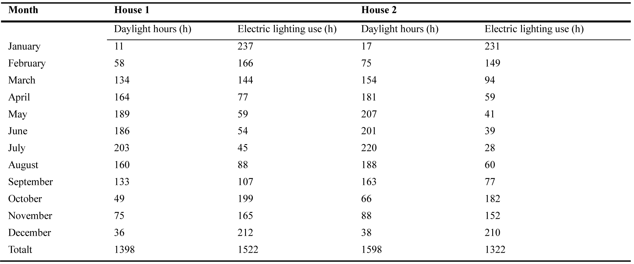
Table 2. Number of daylight hours and electric lighting use hours in houses 1 and 2 for each month.

Table 3

Pair-wise comparison of the percentage of DA per month based on measuring results from the house sensors during 12 months and the two light pipe systems.

Table 3. Pair-wise comparison of the percentage of DA per month based on measuring results from the house sensors during 12 months and the two light pipe systems.

a) Measuring points according to Fig. 3.
b) Significance level at pair-wise comparison of measuring points: *p < 0.05; **p < 0.01; ***p < 0.001; ns = none-significant.

3.2. DA potential

The function of the on/off sensor, which is captured by the s1 sensor is shown in Fig. 7. In analysing the measurement values, it was evident that the built-in time delay function yielded a reduced amount of recorded DA per day. The DA potential (approximatly 67%) in which the time delay function of the on/off sensor and the SSF are accounted is given in Fig. 8.

Figure 7

Illustration of the dusk-dawn sensor function on March 14. At 08.00, the illumination from the light pipes is still insufficient, and the GHI curve is rising but the lights are still on. At 09.15, the GHI curve has risen far enough to cause the sensor to turn off the light.

Fig. 7. Illustration of the dusk-dawn sensor function on March 14. At 08.00, the illumination from the light pipes is still insufficient, and the GHI curve is rising but the lights are still on. At 09.15, the GHI curve has risen far enough to cause the sensor to turn off the light.

Figure 8

Number of potential DA hours between January and July for (a) house 1 and (b) house 2 when the measured data was adjusted for the time delay from the on/off sensor and sensor soiling.

Fig. 8. Number of potential DA hours between January and July for (a) house 1 and (b) house 2 when the measured data was adjusted for the time delay from the on/off sensor and sensor soiling.

3.3. Measured illuminance in the house

The mean illuminance in house 1 was below the illuminance requirement during the first half of January, but this was not the case in house 2 (Fig. 9). The recorded illuminance level range at pig height during February is shown in Fig. 10. The level of daylight increased steadily during the first half year in house 1 to 150 lux, while the increase in house 2 was slightly smaller. The illuminance from the electric lighting remained at a relative constant level initially, but decreased somewhat during April-June. To determine illuminance levels in the houses between 08.00-16.00, a frequency distribution of the illuminance was calculated at pig level (0.7 m above floor level) during January to June from the values of the v1 and s1 sensors (Figs. 11 and 12). The most common frequency range for both houses was from 0 to 160 lux, which corresponded to approximately 82% and 83% of the daylight collection time for house 1 and house 2, respectively.

Figure 9

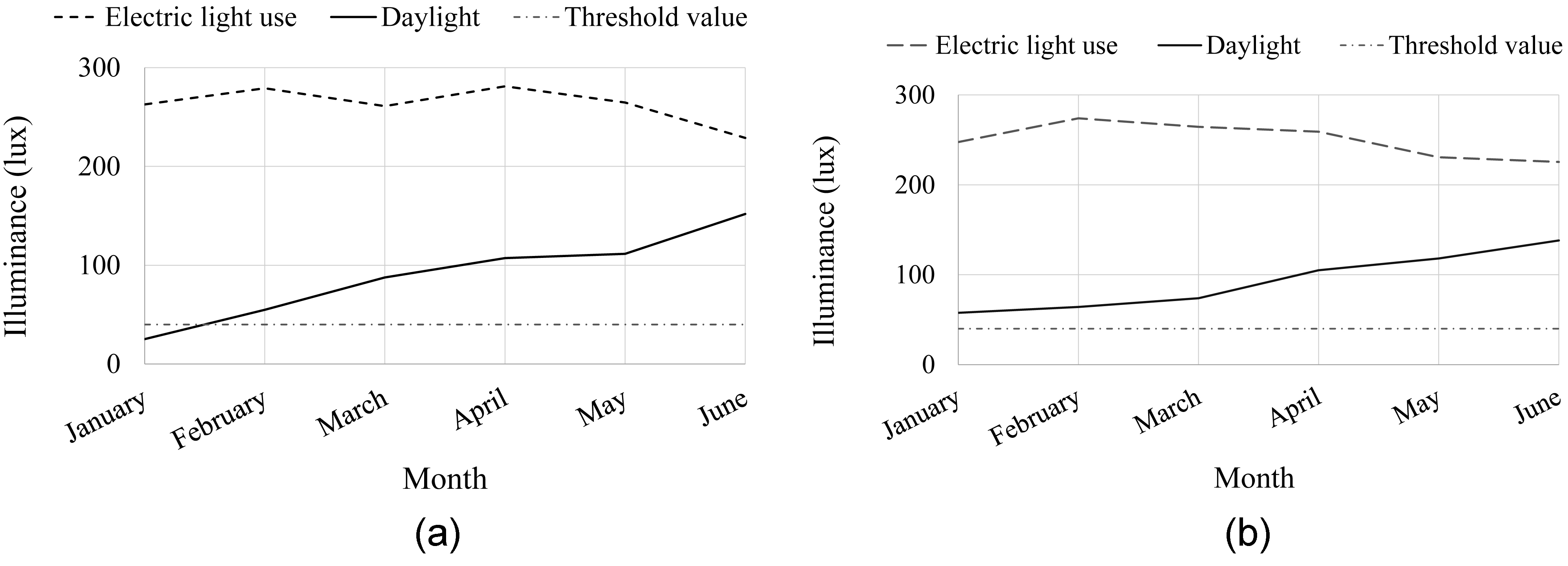
Calculated mean illuminance, based on measurements from sensor s1 and v1 at 0.7 m above floor level, from light pipes and from electric lights between 08.00-16.00 during January to June, where the threshold value was 40 lux (dashed line) for (a) house 1 and (b) house 2.

Fig. 9. Calculated mean illuminance, based on measurements from sensor s1 and v1 at 0.7 m above floor level, from light pipes and from electric lights between 08.00-16.00 during January to June, where the threshold value was 40 lux (dashed line) for (a) house 1 and (b) house 2.

Figure 10

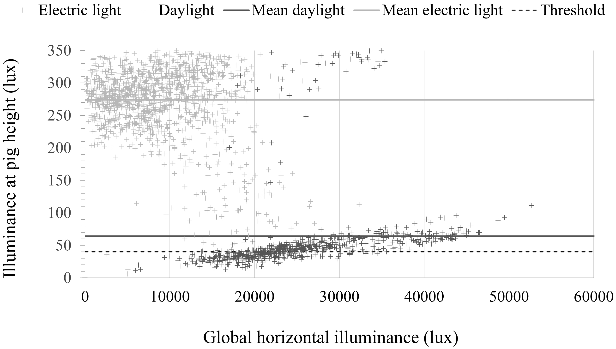
Fig. 10. Example of illuminance levels at pig height (0.7 m) in February for house 2.

Figure 11

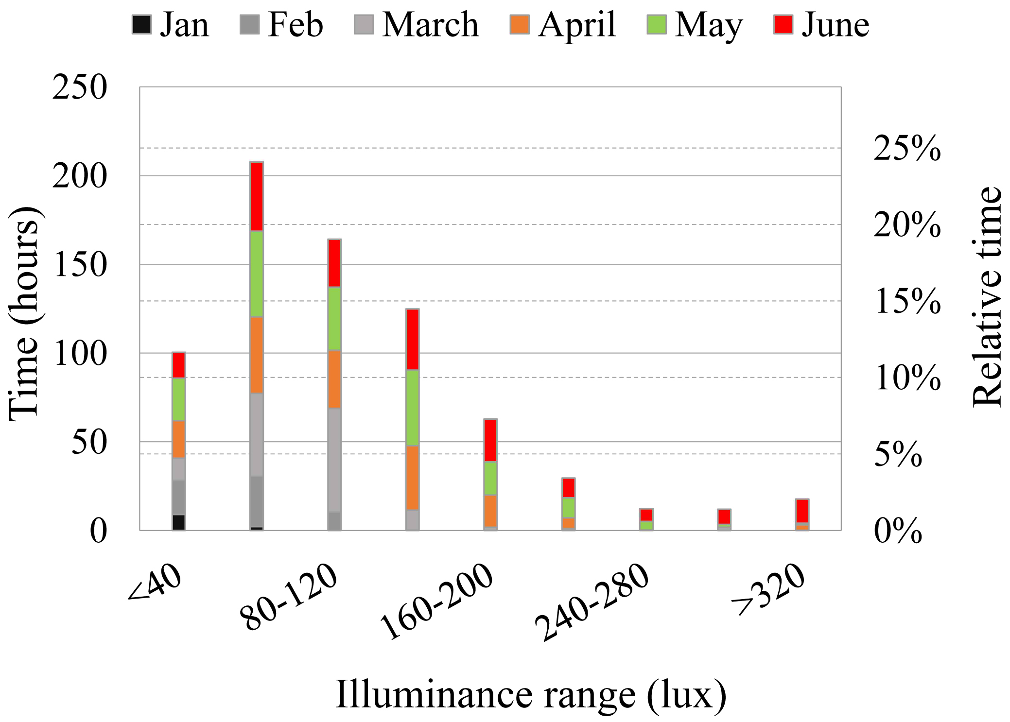
Daylight illuminance frequency distribution at 0.7 m above floor level, based on measured data from sensor v1, in house 1, between 08.00-16.00 hours during January to June.

Fig. 11. Daylight illuminance frequency distribution at 0.7 m above floor level, based on measured data from sensor v1, in house 1, between 08.00-16.00 hours during January to June.

Figure 12

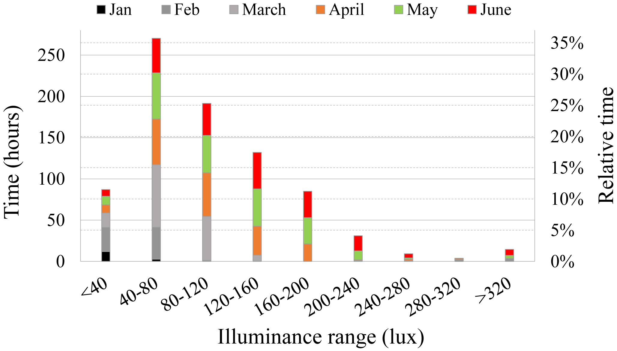
Daylight illuminance frequency distribution at 0.7 m above floor level, based on measured data from sensor s1, in house 2, between 08.00-16.00 hours during January to June.

Fig. 12. Daylight illuminance frequency distribution at 0.7 m above floor level, based on measured data from sensor s1, in house 2, between 08.00-16.00 hours during January to June.

3.4. Daylight distribution and daylight factor

The GHI varied on some occasions although the sky was very overcast, which resulted in only five of nine DF measurements being used from the June recordings. In November, the overcast sky conditions were better. Mean values and SD were calculated for all measurements (n = 96), as shown in Fig. 13. The mean DF range was between 0.03% and 0.56% for the house 1 system and between 0.05% and 0.59% for the house 2 system. Pair-wise comparison of the DF grid at 1.5 m above floor level revealed significant differences for four points, but not for the grid at floor level (Table 4). The SD was lower for house 2 than for house 1, but higher for the measuring point closest to the window in both houses. In general, the light intensity and DF increased with decreasing distance between the measuring point and the light pipe (Fig. 14). At any distance from the light pipes, house 2 generally produced higher DF values.

Figure 13

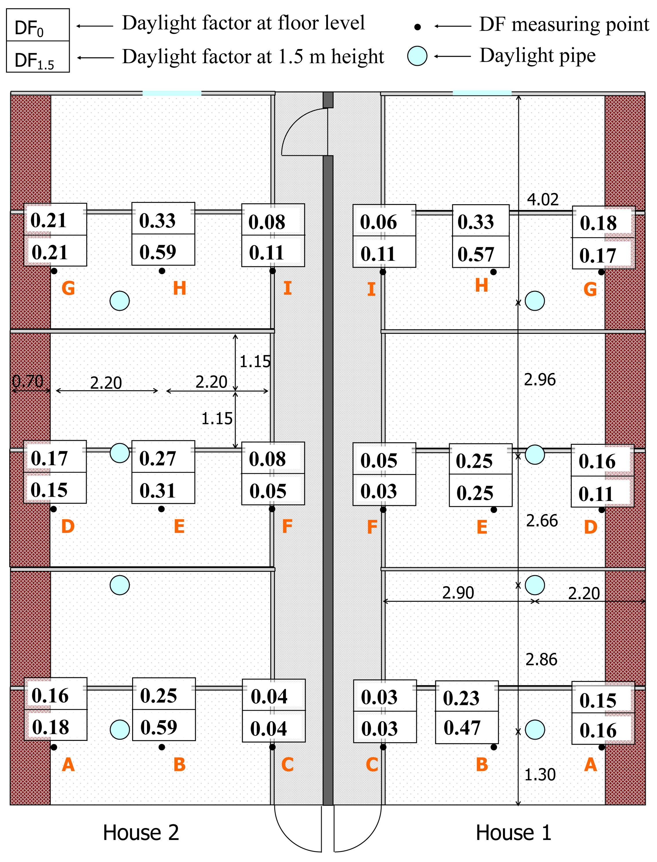
Mean daylight factor (DF, %), for house 1 and house 2 based on measurements conducted in June and November (n=96) at floor level (above) and at 1.5 m above floor level (below in each box for each measurement point), distances in m.

Fig. 13. Mean daylight factor (DF, %), for house 1 and house 2 based on measurements conducted in June and November (n=96) at floor level (above) and at 1.5 m above floor level (below in each box for each measurement point), distances in m.

Table 4

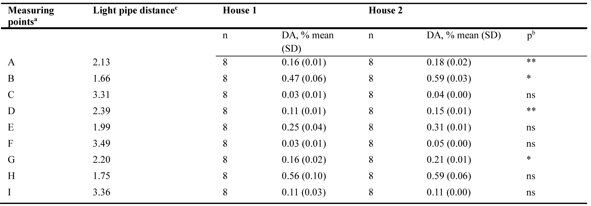
Table 4. Pair-wise comparison of daylight factor (DF, %) at the measuring points 1.5 m above floor level.

Figure 14

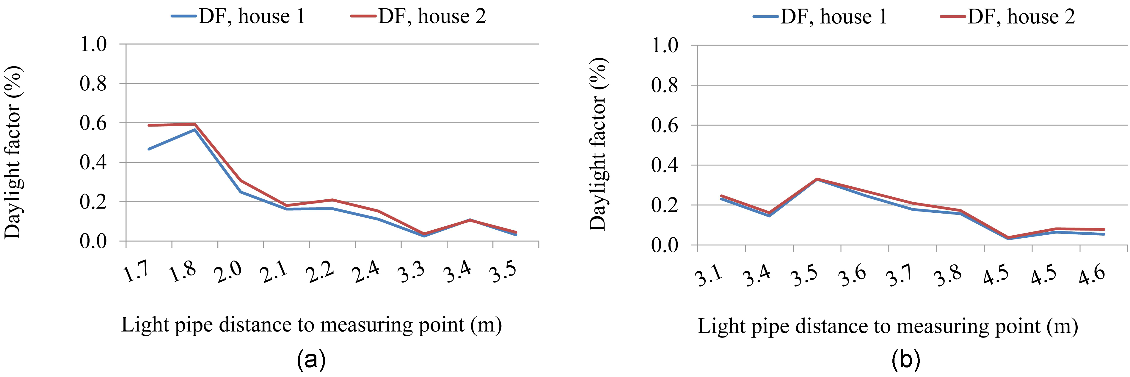
Daylight factor (DF, %) for house 1 and house 2, in relation to distance between light pipe and measuring point for (a) 1.5 m grid above floor level and (b) 0 m grid at floor level.

Fig. 14. Daylight factor (DF, %) for house 1 and house 2, in relation to distance between light pipe and measuring point for (a) 1.5 m grid above floor level and (b) 0 m grid at floor level.

4. Discussion

4.1. Daylight autonomy and illumination

The DA results show that light pipes can offer environmental and energy-efficient daylight without downdraught for animals with low or reduced illuminance level requirements, such as growing pigs, broilers, and laying hens. However, the current low electricity price makes investment in this energy saving potential unprofitable.

The light pipes in house 2 gave higher light output and higher energy saving than those in house 1. This was probably due to many factors, including straight light pipe, higher light pipe reflectance, higher specular reflectance, higher transmittance in the collector and the diffuser, dome collector redirection capacity (useful at Nordic latitudes), etc.

The recorded illuminance ranges in this case were dependent on the relatively low threshold illumination of 40 lux. With a higher threshold set point, i.e. above 40 lux, the most frequent illuminance ranges would have been 40-160 lux according to Figs. 11 and 12, corresponding to 68% and 72% of the daylight collection time for house 1 and house 2, respectively. This also covered the electric illuminance of 80 lux, which was recorded in the houses at 0.85 m above floor level before light pipe installation [27]. An illuminance level of 100 lux, the DA in April onwards (Fig. 9), could be used for spatial orientation in corridors and toilets, with full daylight illuminance at higher solar angles during six months of the year according to [28] and along with complementary lighting for the rest of the year [29]. In all, this would still provide about 33% and 37% of DA for house 1 and house 2, respectively, which was calculated at 0.7 m above floor level, compared with the DA at sensor level.

4.2. Measuring system

The sampling rate used to cope with the high variability of predominantly overcast skies in northern Europe was also used by [20,19]. With logger data averaged both minute by minute and every six minutes, a more detailed measure of sky variability would have been provided. The recorded mean illuminance levels in Fig. 10 are within the same range as light pipe measurements made in the UK with approximately the same pipe length and diameter and point of measurement [20]. The cloud cover during the measuring period, 2013-2014, fell outside the normal range for January, July, and October, with higher cloud cover in January and October but lower in July (Fig. 15). Apart from January, the differences during the period appeared to average out to a normal year.

Figure 15

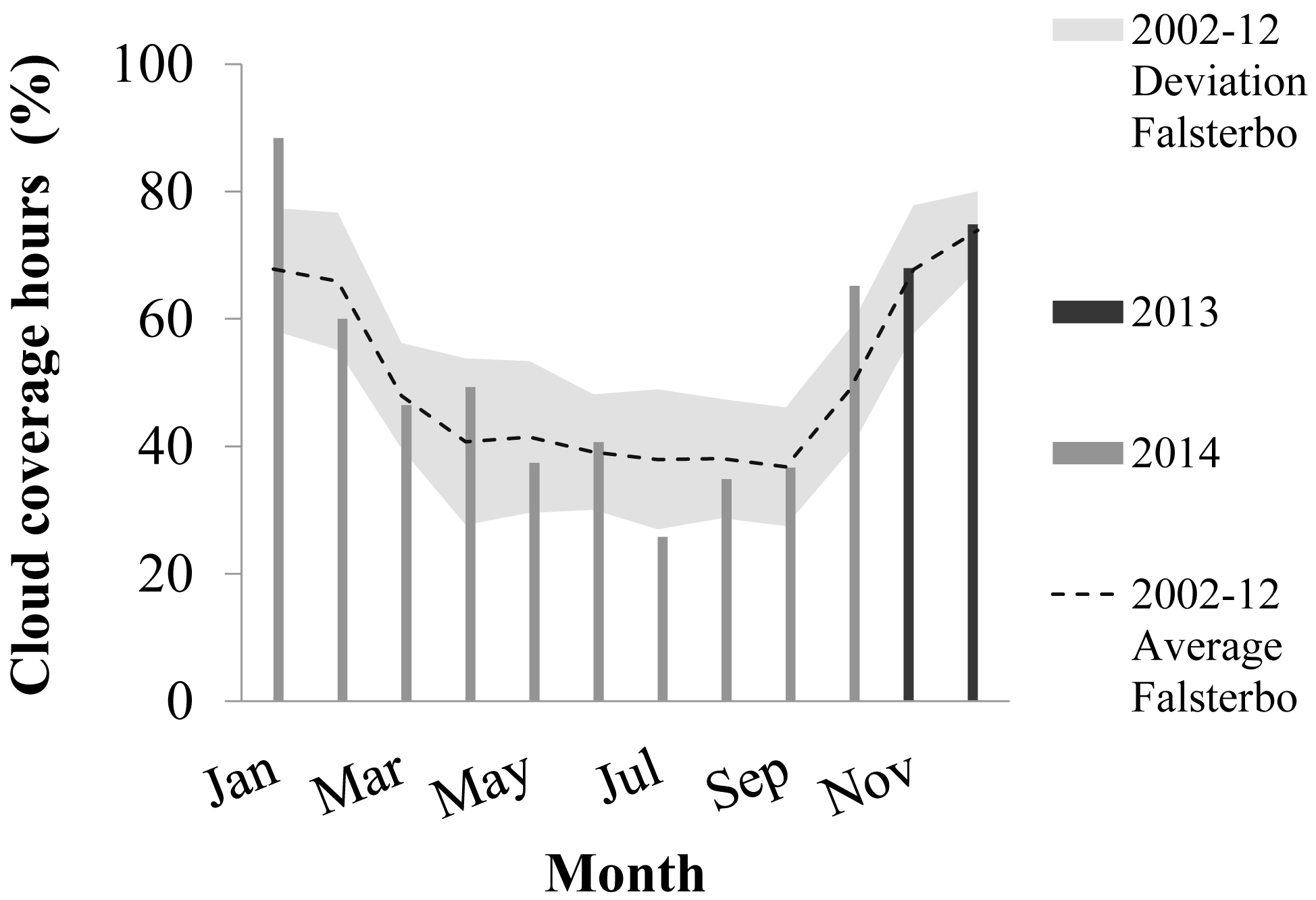
Percentage of hours with 80-100% cloud cover between 06.00 and 18.00 during 2013-2014 at Odarslöv compared with the average cloud cover measured at Falsterbo (55°38'N, 12°82'E) during 2002-2012.

Fig. 15. Percentage of hours with 80-100% cloud cover between 06.00 and 18.00 during 2013-2014 at Odarslöv compared with the average cloud cover measured at Falsterbo (55°38'N, 12°82'E) during 2002-2012.

The error sources based on data from the soiling factor and the on/off sensor (DA potential) were estimated to be approximately 30%. Using the calculated DA potential with a threshold of 40 lux, the DA corresponded to approximately 67% for both light pipe systems. Recalculating the DA potential for a threshold above 40 lux, it would correspond to approximately 54% and 57% for house 1 and house 2, respectively, with the exception of differences in illuminance ranges with a higher sampling rate. The sensor measuring range was chosen according to normal illuminance. With a threshold of 40 lux, the measuring sensors operated close to their stated accuracy level. This could mean that sensor errors for low illuminance conditions would be larger. However, recorded data showed a linear response to increased illuminance (Fig. 10).

4.3. Daylight distribution and daylight factor

In conventional office spaces, the minimum requirement for horizontal illuminance on work surfaces is 500 lux [30]. Such values are generally supplied solely by daylight in areas where DF ≥ 5%, while electric light may be required for 2% ≤ DF < 5%, and daylight contribution is considered negligible in areas with DF < 2% [24]. The mean DF values measured in pig houses 1 and 2 and at both sensor heights (0 and 1.5 m) were lower than 1%. With a low target illuminance level and the fact that light pipes have a visible transmittance that is decidedly lower than that of a common glazed window, a low DF was expected. However, the target horizontal illuminance was also much lower than the standard for humans in offices; therefore, the daylight contribution was conceivably relevant for houses with growing animals.

The statistical DF data together with the information in Fig. 14 showed that the illuminance at the two grid levels varied. A possible cause of this is that the grid points received illuminance from more than one light pipe and that the light pipe placement in relation to the pen dividing walls perhaps blocked the path of the light rays. Moreover, there were differences between the characteristics of the light distribution through the diffuser. These parameters explain why the DF values did not vary as much from ground to 1.5 m when the grid points were far from the light pipes. The corresponding variation was much higher when the grid points were closer to the pipe. Although the grid points A, B, and C were almost symmetrical to points G, H, and I, and there were differences in DF. This was due to the presence of the window on the north wall, which could be an indication of the reliability of DF calculation.

In general, the illuminance and DF were highest close to the light pipe centre line, just above the animal feeding troughs, and decreased with distance from the centre line. The illuminance was at its lowest along the dunging area, while the resting area, with its isolated cover, had a reduced illuminance at floor level. This is not entirely in accordance with pig preferences [10]. However, it shows the importance of light pipe design and diffuser characteristics for light pipe placement to satisfy pig light preferences.

4.4. Design considerations

The electric lighting use in animal production buildings for farm personnel is generally short, and the main users are the animals. With the annual DA results obtained here, the amount of electricity used for lighting purposes in farm buildings for growing pigs, broilers, and laying hens could be reduced. Combining light pipes with dimmable LED lights in periods of weak DA could reduce the electricity use for lighting to an even lower level [29].

With higher indoor temperatures, energy savings through dim daylight delivered by light pipes, instead of windows with low insulation characteristics, could be even more beneficial in poultry production. Light pipes provide a non-flickering, continuous spectrum of daylight, which could enhance visual communication and influence the physical system for the birds [31]. Daylight levels obtained by light pipes during the summer period could be too high, but could be reduced by built-in automatic shading devices [32,33].

Solar angle and sky clearness are key parameters for light pipe performance [15]. For that reason, animal buildings with low pitched roofs of 15-22° are well suited for low solar angles in the northern and southern hemisphere. As for pig health status, the pigs produced at Odarslöv had a considerably lower defect score than the slaughterhouse average in both 2013 and 2014.

Based on the DA potential results, light pipes could offer an energy saving potential of approximatly 55% if lower daylight illumination levels could be considered in periods with lower solar angles, with complementary lighting in corridors and toilets for maintenance staff. A saving of 50% of electric lighting in the animal production sector would represent at least 36 GWh, corresponding to 2520 t CO₂ per year for Sweden [5,34].

5. Conclusions

This study evaluated whether reduced electricity use for lighting purposes in farm buildings could be achieved by increased DA from two light pipe systems and examined the functionality of these systems in the daily operation of an animal house with a soiling environment. Daylight was measured in two identical pig houses that were fitted with four light pipes each, with three continuously measuring sensors in each house and an outdoor sensor during 2013 and 2014. If the illuminance fell below 40 lux during 08.00-16.00, a sensor turned on the electric lighting, and the electricity use was recorded. Data analysis was carried out monthly based on the conditional function that the electricity use should be zero. The DF was manually measured on two occasions with no pigs in the houses.

The mean total annual DA was 48% for house 1 (Velux^®) and 55% for house 2 (Solatube^®), with mean DA of approximately 51% and 57% in the first half-year and 45% and 52% in the second half-year for house 1 and house 2, respectively. Light pipes for house 2 delivered significantly more DA than those in house 1. The most common illuminance frequency range for both houses was between 0 and 160 lux, corresponding to approximately 82% and 83% of the daylight hours for house 1 and house 2, respectively. Based on differences recorded at four points for the DF grid at 1.5 m above floor level, house 2 had higher DF values, indicating that its light pipe system achieved more effective light collection and distribution, even under overcast sky conditions.

With the annual DA results, considerable electric energy savings could be achieved in pig, broiler, and laying hen production by increased use of daylight in farm buildings. One advantage for the animals is that they would be exposed to a non-flickering, continuous spectrum of daylight, the natural light source under which all species have evolved during millions of years. For staff working in animal houses, light pipes could offer an energy saving potential, especially if combined with dimmable LED lights and if lower daylight illumination levels were accepted in corridors and toilets in periods with lower solar angles. However, this investment would only be financially viable with a higher electricity price than at present.

Future research questions regarding light pipes could address (e.g., diffuser and light pipe specular reflectance durability in relation to environmental gases in animal houses and light pipe function in relation to fire safety).

Acknowledgements

The authors gratefully acknowledge financial support from the Swedish Energy Agency (36459-1), the Region Skåne Fund for Environmental Studies (M 080) and the Swedish Farmers Accident Insurance Fund (H132-0027-SLO). We also thank Mats Olsson and Thomas Nilsson for help in carrying out the experiments and Jan-Eric Englund for statistical advice.

Contributions

H. v. Wachenfelt conceived the study and wrote the manuscript with input from all the authors. N. Gentile and K.-H. Jeppsson performed the pig house measurements. V. Vakouli processed results together with A. Pacheco Diéguez’, and M.-C. Dubois contributed to the results analysis. All the authors discussed the results.

References

IEA, Light’s labour cost, International Energy Agency (IEA), France, 2006.
SJV Swedish Animal Welfare Agency, Swedish Board of Agriculture, SJVFS 2014:31 L100, in Swedish, Jordbruksverket, 2014.
CEC, Commission Directive 2001/93/EC of 9 November 2001 amending Directive 91/630/EEC: Laying down minimum standards for the protection of pigs, Commission of the European Communities, Brussels, Belgium, 2001.
M. Edström, O. Pettersson, L. Nilsson, and T. Hörndahl, Energy in farming, in Swedish: JTI-rapport 342, Swedish Institute of Agricultural and Environmental Engineering, Uppsala, 2005.
T. Hörndahl, Energy consumption in farm buildings, in Swedish: LTJ report 145, Swedish University of Agricultural Sciences, Dept. of Biosystems and technology, Alnarp, 2007.
P. Dehoff, The impact of changing light on the well-being of people at work, in: Right Light, 2002, 374–351.
S. Harteb Puleo and R. Leslie, Some effects of sequential experience of windows in human response, Journal of the Illuminating Engineering Society 20 (1991) 91–99. http://dx.doi.org/10.1080/00994480.1991.10748928.
G.M. Figueiro, Daylight and Productivity - A Field Study, in: ACEEE Summer Study on Energy Efficiency in Buildings, American Council for an Energy-Efficient Economy, Washinngton DC, 2002.
T. Ashkenazy, H. Einat and N. Kronfeld-Schor, Effects of bright light treatment on depression- and anxiety-like behaviors of diurnal rodents maintained on a short daylight schedule, Behavioral Brain Research 201 (2009) 343–346. http://dx.doi.org/10.1016/j.bbr.2009.03.005
N. Taylor, N. Prescott, G. Perry, M. Potter, C. Le Sueur, and C. Wathes, Preference of growing pigs for illuminance, Applied Animal Behaviour Science 96 (2006) 19–31. http://dx.doi.org/10.1016/j.applanim.2005.04.016
K.N. Gelatt (Ed.), Veterinary Ophthalmology, 3rd ed. Lippincott, Williams and Wilkins, Philadelphia, 1998.
M.J. Chandler, P.J. Smith, D.A. Samuelson, and E.O. Mackay, Photoreceptor density of the domestic pig retina, Veterinary Ophthalmology 2 (1999) 179–184. http://dx.doi.org/10.1046/j.1463-5224.1999.00077.x
E.M.A.M. Bruininx, M.W. Heetkamp, A. Bogaart, C.M.C. van der Peet-Schwering, A.C. Beynen, H. Everts, L.A. den Hartog, and J.F.W. Schrama, A prolonged photoperiod improves feed intake and energy metabolism of weanling pigs, Journal of Animal Science 80 (2002) 1736–1745.
S.R. Niekamp, M.A. Sutherland, G.E. Dahl, and J.L. Salak-Johnson, Photoperiod influences the immune status of multiparous gestating sows and their piglets, Journal of Animal Science 84 (2006) 2072–2082. http://dx.doi.org/10.2527/jas.2005-597
T. Zhang and T. Muneer, Mathematical model for the performance of light-pipes, Lighting Research and Technology 32 (2000) 141–46. http://dx.doi.org/10.1364/OE.20.009004
J. Mohelnikova, Tubular light guide evaluation, Building and Environment 44 (2009) 2193–2200. http://dx.doi.org/10.1016/j.buildenv.2009.03.015
A. Nilsson, A. Daylighting Systems: Development of Techniques for Optical Characterization and Performance Evaluation, Acta Universitatis Upsaliensis, Digital Comprehensive Summaries of Uppsala, Dissertations from the Faculty of Science and Technology, Uppsala, 2012.
E. Kjellsson, Solar heating systems for electricity heated houses, Report number U02:86, Vattenfall AB, 2002.
H. Danny, K. Ernest, K. Cheung and C. Tam, An analysis of light-pipe system via full-scale measurements, Applied Energy 87 (2010) 799–805. http://dx.doi.org/10.1016/j.apenergy.2009.09.008
X. Zhang, T. Muneer, and J. Kubie, A design guide for performance assessment of solar light-pipes, Lighting Research and Technology 34 (2002) 149–168. http://dx.doi.org/10.1191/1365782802li041oa
V. Lo Verso, A. Pellegrino, and V. Serra, Light transmission efficiency of daylight guidance systems: An assessment approach based on simulations and measurements in a sun/sky simulator, Solar Energy 85 (2011) 2789–2801. http://dx.doi.org/10.1016/j.solener.2011.08.017
I. Edmonds, G. Moore, G. Smith, and P. Swift, Daylighting enhancement with light pipes coupled to laser-cut light-deflecting panels, Lighting Research and Technology 27 (1995) 27–35. http://dx.doi.org/10.1177/14771535950270010101
N. Gentile, H. Håkansson, and M.C. Dubois, Lighting control systems in individual offices at high latitude: measurements of lighting conditions and electricity savings, in: 7th International Conference on Energy Efficiency in Commercial Buildings, 2013, 333–344, Germany.
CIE, Spatial distribution of daylight-CIE standard general sky, CIE S 011, Vienna, 2003.
Minitab, available online: http://www.minitab.com. (accessed on 1 Mar 2015).
SAS Institute Incorp, Base SAS® 9.3 Procedures Guide. Cary, NC, SAS Institute Incorporated, 2011.
K.H. Jeppsson, D. Nilsson, H. von Wachenfelt, and T. Hörndahl, Lighting design in animal buildings with DiaLux and a quantitative assessment of lighting environment on pasture vs indoors for cattle, in Swedish, LTJ-report 2013:34, Alnarp, 2014.
P. Tregenza and M. Wilson, Daylighting: Architecture and Lighting Design, Routledge, 2011.
L. Bellia, F. Fragliasso, and A. Pedace, Evaluation of daylight availability for energy savings, Journal of Daylighting, 2 (2015) 12–20. http://dx.doi.org/10.15627/jd.2015.2
CEN/TC, PrEN 15193: Energy performance of buildings - Energy requirements for lighting, Brussels, 2007.
N. B. Prescott, C. M. Wathes, and J. R. Jarvis, Light, vision and the welfare of poultry, Animal Welfare 12 (2003) 269–288.
Solatube International, Inc., Available online: http://www.solatube.com/commercial/product-catalog/brighten-up-series/index.php (accessed on 10 Feb 2014).
Velux, VELUX sun tunnel material properties for SGG Bioclean, Available online: http://www.velux.se (accessed on 1 Feb 2015).
P. Börjesson, L. Tufvesson, and M. Lantz, Life Cycle Assessment of Biofuels in Sweden, Report 70, in Swedish, Environmental and Energy Systems Studies, Lund University, Lund, Sweden, 2010.

Get PDF (3.35 MB)

SHARE ON