The Effect of Sky View Factor on Air temperature in High-rise Urban Residential Environments

^a Energy and Architecture, Architecture Department, Faculty of Technology and Engineering, Ilam University, Ilam, Iran
^b Architecture Department, Faculty of Technology and Engineering, Ilam University, Ilam, Iran

* Corresponding author.
golnar.baghaeipoor@gmail.com (G. Baghaeipoor)
n.nasrollahi@ilam.ac.ir (N. Nasrollahi)

History: Received 2 June 2019 | Revised 17 August 2019 | Accepted 19 August 2019 | Published online 30 August 2019

Citation: Golnar Baghaeipoor, Nazanin Nasrollahi, The Effect of Sky View Factor on Air temperature in High-rise Urban Residential Environments, Journal of Daylighting 6 (2019) 42-51 http://dx.doi.org/10.15627/jd.2019.6

Figures and tables

Figure 1
Figure 2
Figure 3
Table 1
Table 2
Figure 4
Figure 5
Figure 6
Figure 7
Figure 8
Table 3
Figure 9
Table 4
Table 5

Abstract

Urban geometry is defined by the height, length, width, and distance of buildings, which affect the urban environment and its microclimate, especially a high-rise and high-density urban environment, such as Tehran. In this regard, the Sky View Factor (SVF) may often be a desirable criterion in identifying the interaction between urban geometry and the air temperature in densely populated areas. The research aim was to investigate the SVF in an urban microclimate of a high-rise residential complex and to evaluate its effect on air temperature. To do so, a case study of the Atisaz in Tehran as a high-rise urban residential complex was selected as the fundamental study model of this research. The selected configuration was simulated and analyzed using the ENVI-met model. In addition, the effects of the SVF value on air temperature are discussed throughout this paper. SPSS software was used to correlate, analyze, and construct an accurate relationship between air temperature and SVF during the hottest and coldest days of the year. The obtained results showed that there is a direct relation between SVF and air temperature during the day as well as an inverse relation at night. Furthermore, there was a small difference in air temperature for dense and semi-dense spaces in the high-rise residential complex.

Keywords

Sky view factor, Urban geometry, Residential complex, High-rise buildings

1. Introduction

Sky exposure is an ongoing concern. From an environmental perspective, reduction in sky exposure can lead to decrease in daylight access for residents, especially in high-density urban area, resulting in compromised visual comfort and requiring artificial lightening even during daytime [1]; additionally, from a psychological point of view, reducing sky exposure threatens the mental comfort of the residents. Sky exposure provides good access to light in urban open spaces as well as inside buildings [1]. In addition, Exposure to natural light has a positive effect on the physical and mental health of people [2,3]. Excessive sky exposure and solar radiation could have negative impacts because they increase the need for mechanical cooling and ventilation and subsequently energy consumption [1]. Therefore, sky exposure is a significant parameter in dense cities [1].

There are various methods to obtain the SVF value. In 1981, Oke [4] suggested the geometrical method of calculating SVF using simple geometric compositions; in reality, the geometry of urban buildings is asymmetric and their dimensions are limited. Considering such a constraint, Johnson and Watson [5] revised Oke’s theory as well as equations and introduced the SVF value for more realistic situations in 1984. The fish-eye photograph is another method of SVF calculation [6,7]. Anderson [8] was the first to implement photography techniques to measure SVF in 1964. He used photographic calculations to estimate the amount of sun light radiation on his shelter while residing in a jungle, then the photographic method became a popular way to evaluate SVF in urban climates. In 1980, Steyn [9] published an article explaining a manual method for the evaluation of the fish-eye images; however, Johnson and Watson [5] proposed a revised version of Steyn’s formula in 1984. Barring and his colleagues [10] digitalized the fish-eye method with a recording camera in 1985, and consequently, advances in saving the camera images by Steyn et al. [11] in 1986 took place in one frame. Eliasson [12] investigated the effects of SVF on the daily changes in air temperatures and surfaces in 1990. SVF was calculated with two new methods of digitalized images using commercial software in 2000 [13]. For the first method by using IDRISI software, SVF was calculated in forest areas by scanned fish-eye images. For the second method by using infrared sensors dependent to simultaneously measured air temperature and road surface temperature, SVF was calculated along the road [13].

Examining GPS signals is another method of measuring SVF, which was proposed by Chapman et al [14] with the prime goal of performing an online calculation of SVF using proxy data in 2002. The aforementioned method was developed further for a real-time calculation by Chapman and Thornes [15]. The software method is widely used, which offers a quick way to calculate SVF. The vector and raster algorithms are highly implemented in this method. The vector algorithm uses the proposed geometric relationship by Oke [16] in 1987, while the raster method takes advantage of the shadow casting algorithm introduced by Richens and Ratti [17] in 1999. The shadow casting algorithm utilizes a precise digital database of height angles, digital elevation model (DEM), and constructs a pattern of a building’s shadow; however, in 2005, this algorithm was modified and developed further by Lindberg [18] for SVF calculations. On the one hand, it has been proven by Gal et al [19] in 2009 that the raster algorithm performs at a faster rate in contrast with the vector algorithm, but on the other hand, Bernard et al in 2018 designed a new vector-based SVF calculation tool, OrbisGIS, with higher accuracy and computational performance compared to the ones of an existing raster based algorithm, SAGA-GIS [20]. In [21], Jianming et al introduced a new computational framework (SVF Engine) which derives SVF from a wide variety of city models. For evaluating the SVF Engine performance, they used OAP3D, a new photogrammetry-based 3D city model, and calculated the SVF for 30 different locations. They compared the SVF estimates with those from the street view panoramas and found the SVF estimates obtained using both methods closely match each other with correlation coefficient of 0.99. Mirzaee et al [22] proposed a new algorithm to calculate average SVFs of hypothetical neighborhoods based on using two geometric characteristics: building density of the area and average height of the buildings. This method is fast, simple, and free of 3-dimentional shapefiles of the area [22]. It should be noted the effects of plantation and inclined surfaces in the aforementioned methods are not considered or discussed thoroughly [23-25].

Various studies have been conducted regarding the relationship between air temperature and SVF. Simulations carried out by Oke [26] and his colleagues in 1991 showed that the difference in SVF between the suburbs and the city can produce difference in temperature between 5-7 °C, although parameters such as heat released by human activities and the thermal properties of materials increase the heat island effect in a building overnight. Eliasson’s work [27] in 1996 provided significant results showing that there is no statistical connection between the geometry of urban straits and air temperature in the central districts of Goteborg. Barring et al [10] in 1985 in Sweden concluded that the air temperature is not highly dependent on urban canyon geometry; however, Yamashita et al [28] in 1986 in Japan found a firm relationship between air temperature and SVF in the cities of Fuchu and Higashimurayama. Karlsson [29] in 2000 presented a relation between air temperature, pure solar radiation, and SVF in forests. Svensson [30] in 2004 showed that there is a strong relationship between air temperature overnight and SVF, and both parameters of land use and SVF affect air temperature variations in urban environments. Recent results show that this relationship is less clear. According to a comprehensive review by Unger [31] in 2004, several reports on the same urban areas showed strong, poor, and insignificant interactions between SVF and the urban heat-island (UHI). In his new approach, comparing the average geometry and air temperature variations, the clarity of the relationship between SVF and air temperature has been confirmed [32].

In 2003, Atkinson [33] simulated the intensity of the UHI in an ideal urban structure using a numerical method. After conducting controlled tests, he found that the absence of SVF in the urban heat islands would decrease the air temperature by 0.3° C in the morning. The value of SVF in this research was 1 for rural areas and 0.4 for urban areas; however, other SVF values have not been studied.

Steemers et al [34] in 2004 analyzed the relation between SVF and air temperature fluctuations. In a study in Cambridge, which included measuring the air temperature and obtaining data in the morning during the spring, they found that increasing SVF results in a higher rate of air temperature fluctuations of higher degrees. Blankenstein and Kuttler [35] stated that because SVF cannot describe thermal properties, the diversity within the urban heat island alone cannot be predicted by SVF. In 2010, Bourbia and Boucheriba [36] studied the effect of designing streets on micro-climates in a highly dense city in North Africa with hot and dry climates. The geometry of streets was introduced by the SVF which is obtained through fish-eye images and H/W proportions. Seven stations within the SVF range of 0.076- 0.58 were analyzed. July was chosen and measured as the warmest month of the year. A comparison of the average daily air temperature and SVF showed that increasing SVF results in increasing air temperature.

Bourbia and Awbi [37] studied the effect of the height to width ratio (H/W) and SVF in a building cluster on the outdoor air temperature and surface temperature in Algeria and concluded that by controlling SVF and street designs, increasing temperatures can be prevented in urban canyons. In 2004, Giridharan et al [38] discussed the effects of SVF on UHI during the day on Hong-Kong residential expansions. Their analytical research of a small scale included residential buildings with SVF values of 0.373, 0.473, and 0.470. A multi-variable analysis showed that the regression coefficient of SVF for UHI during the day starting at 1.5°C could be positive or negative.

The subsequent research of Grridharan [39] in 2007 expanded the fish-eye is in the range of 0.11 and 0.59. This study showed that during clear days in the summer, all 12 variables, including SVF, surface reflection, wind speed, and etc. could explain the change in the UHI during the day.

Most of the studies have used the photographic method thus far [10,27,36]. The obtained results of such studies are inconsistent because SVF in urban canyons has different effects on the street temperature at the surface level. This effect could be either positive [36,40], negative [12] or neutral [41]. There are similar findings by Unger [31] and Upmanis [42]. Yang and Li in 2015 applied a three-dimensional Model for Urban Surface Temperature (MUST) to estimate the importance of urban geometry on urban albedo and street surface temperature, with a focus on the impact of building density and building height heterogeneity [32].

Overall, these studies have shown the research emphasis on the effect of SVF on air temperature in urban areas. However, a comprehensive research that investigate the relation between air temperature and SVF on a continuous zone has not been conducted yet in an arid climate. Therefore, the objective of this study is to identify and to discuss the relationship between air temperatures and SVF in a high-rise urban residential environment for two important days of the year—the hottest and coldest days—to determine how it impacts air temperatures within a residential site. Hence, this research can help designers to consider the effect of SVF and air temperature for different high-rise residential zone—open, semi-open, semi-dense, and dense.

The high-rise residential complex of Atisaz consists of 23 towers, 12-31 stories, in an area of 15.5 hectares that are located in the northwest of Tehran. The general view and location map of the residential complex are presented in Fig. 1 [41,44].

Figure 1

Fig. 1. (a) A general view and (b) a location map of Atisaz residential complex [41,42].

2. Research methodology

In this research, the simulations have been done by using ENVI-met version 4.0 [45]. ENVI-met is a three-dimensional grid based microclimate model, designed to simulate complex surface-vegetation-air interactions in the urban environment. ENVI-met as a dynamic simulation tool for microclimate analysis [46] was developed by Michael Bruse at the Rurh University of Bochum [47]. Based on the fundamental laws of fluid dynamics and thermodynamics, ENVI-met can simulate the cycle of major climatic variables involving air and soil temperature and humidity, wind speed and direction, radiative fluxes etc. Two main input files are required for the simulations: the area input file, in which the building layout, vegetation, soil type, receptors (i.e. specific grids in the ENVI-met model) and project location parameters are defined and the configuration file, containing simulation settings regarding initialization values for meteorological parameters, definition of output folder names and timings [48].

2.1. Validation of ENVI-met

According to [48-50], In many previous studies, the validation of ENVI-met results has been done by comparing the results of simulation and field measurement. The results of these studies indicate that the software simulates the air temperature and SVF with proper accuracy. Additionally, in this research for validating ENVI-met, simulated and measured results related to July 22th, 2019 were compared. On-site monitoring was carried out exactly at the same conditions that simulation was performed. The air temperature data were measured by BENETECH GM 1365 data logger (accuracy: ±0.3°C, range: -30-80°C) which was protected by a white shield to minimize the effect of radiation (Fig. 2).

The coefficient of determination (R2) between the simulation results and measurements is equal to 0.9141 (Fig. 3) and based on the previous researches [49,51], simulation results in this study have an acceptable level of accuracy.

Figure 2

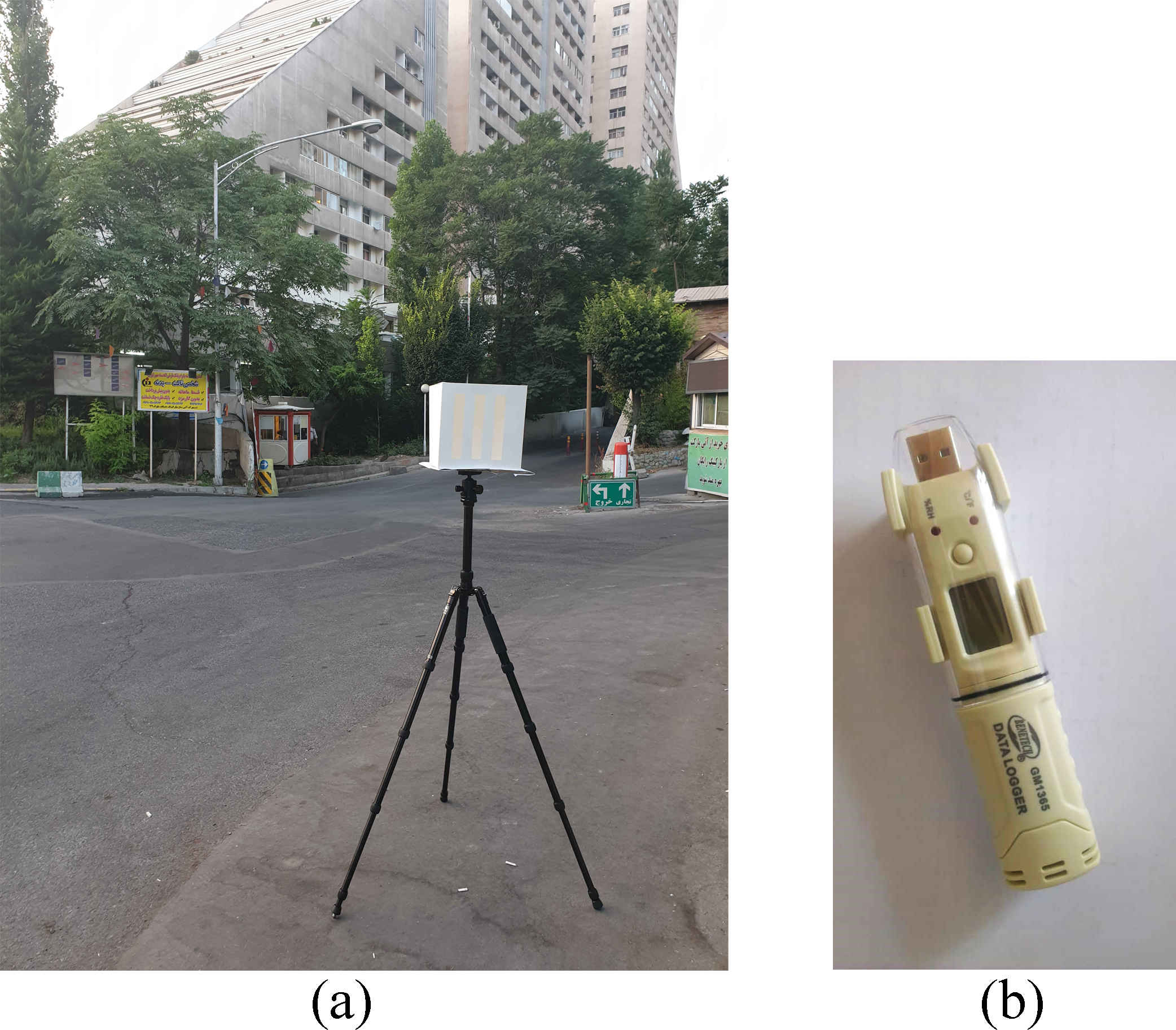
Fig. 2. (a) and (b) Weather data logger for measuring air temperature and relative humidity to validate ENVI-met software.

Figure 3

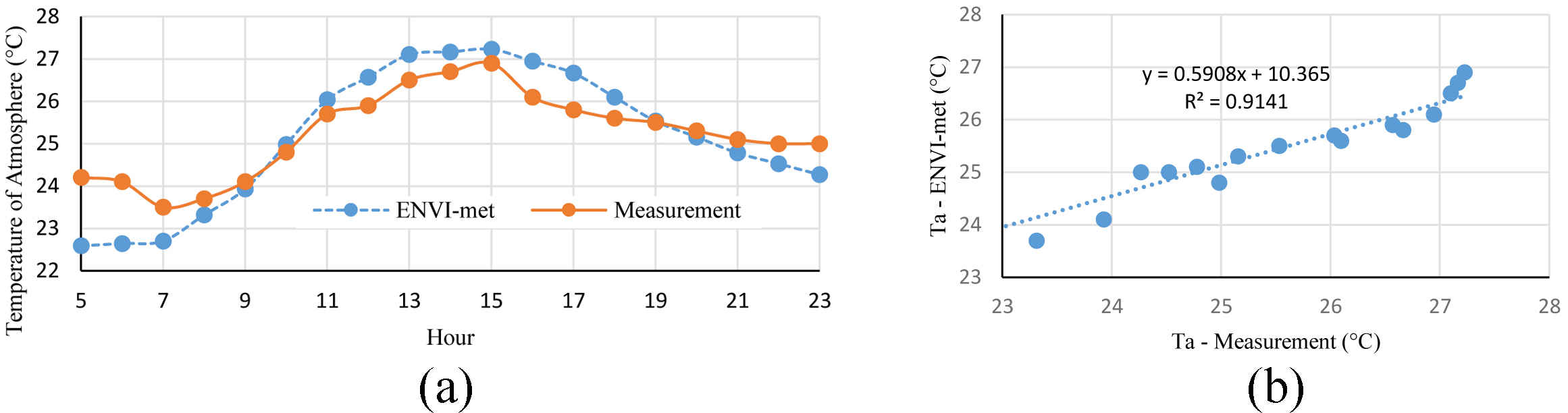
Fig. 3. (a) and (b) A comparison of the measured and simulated air temperatures.

2.2. Case Study

As the case study, the site plan of the Atisaz has been simulated by ENVI-met, and the SVF value as well as the air temperature at different points of the site plan are calculated. Table 1 shows the data for creating 3-D model of Atisaz complex.

Table 1

Table 1. 3-D model data.

Table 2 represents the initial meteorological data which is used as input data for simulation. The simulations were performed for a time period starting of 4:00 h to 24:00 h for two days of the year—the hottest and the coldest days. It should be noted the initial potential air temperature is extracted from the Shemiran weather station, which is based on the average air temperature for the hottest and coldest day in the recent 30 years [52]. Shemiran weather station and Atisaz complex are at the same meters above mean sea level and geographical location.

Figure 4 presents two perspective views and a two-dimensional map of Atisaz which were simulated by ENVI-met. The correlation between air temperature and SVF during each hour of the two days of the year—the hottest and the coldest days— were analyzed in terms of a variance analysis and a regression analysis using the statistical software of SPSS.

Table 2

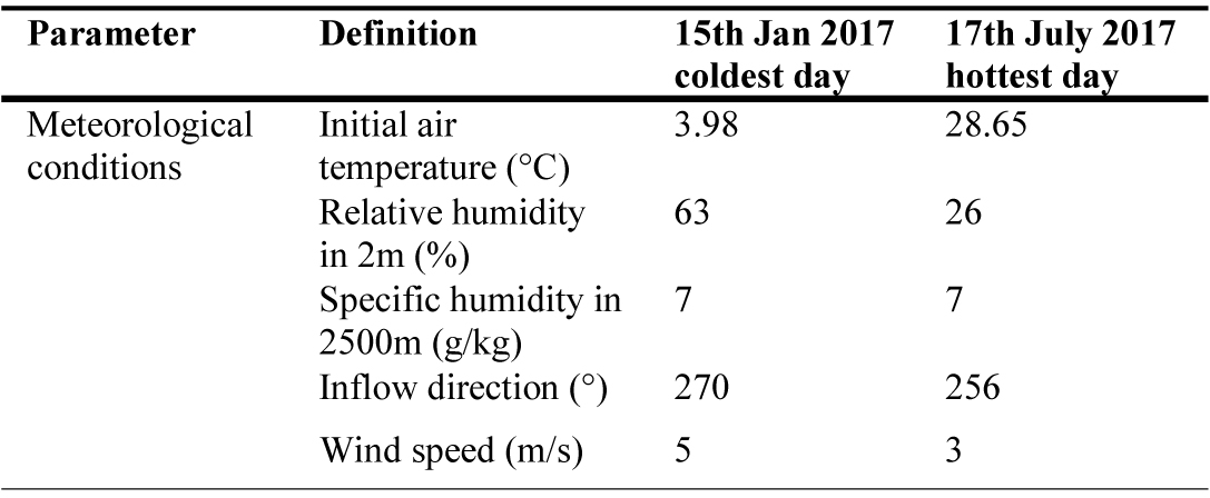
Table 2. Initial meteorological conditions.

Figure 4

Fig. 4. (a) Perspective views and (b) a 2D map of the Atisaz complex simulated by ENVI-met.

3. Design process using the simulation software of ENVI-met

The maximum and minimum values of SVF shown in the site plan of the Atisaz (Fig. 5) are 0.98 and 0.12, respectively. It should be noted that the area with SVF value between 0.8 to 1—pink and purple area—is an empty open space. To determine the effects of SVF on air temperature, the thermal maps of the hottest day of the year at different hours were calculated, and the air temperature counters for some hours are shown on the coldest and hottest days of the year (Figs. 6 and 7).

Figure 5

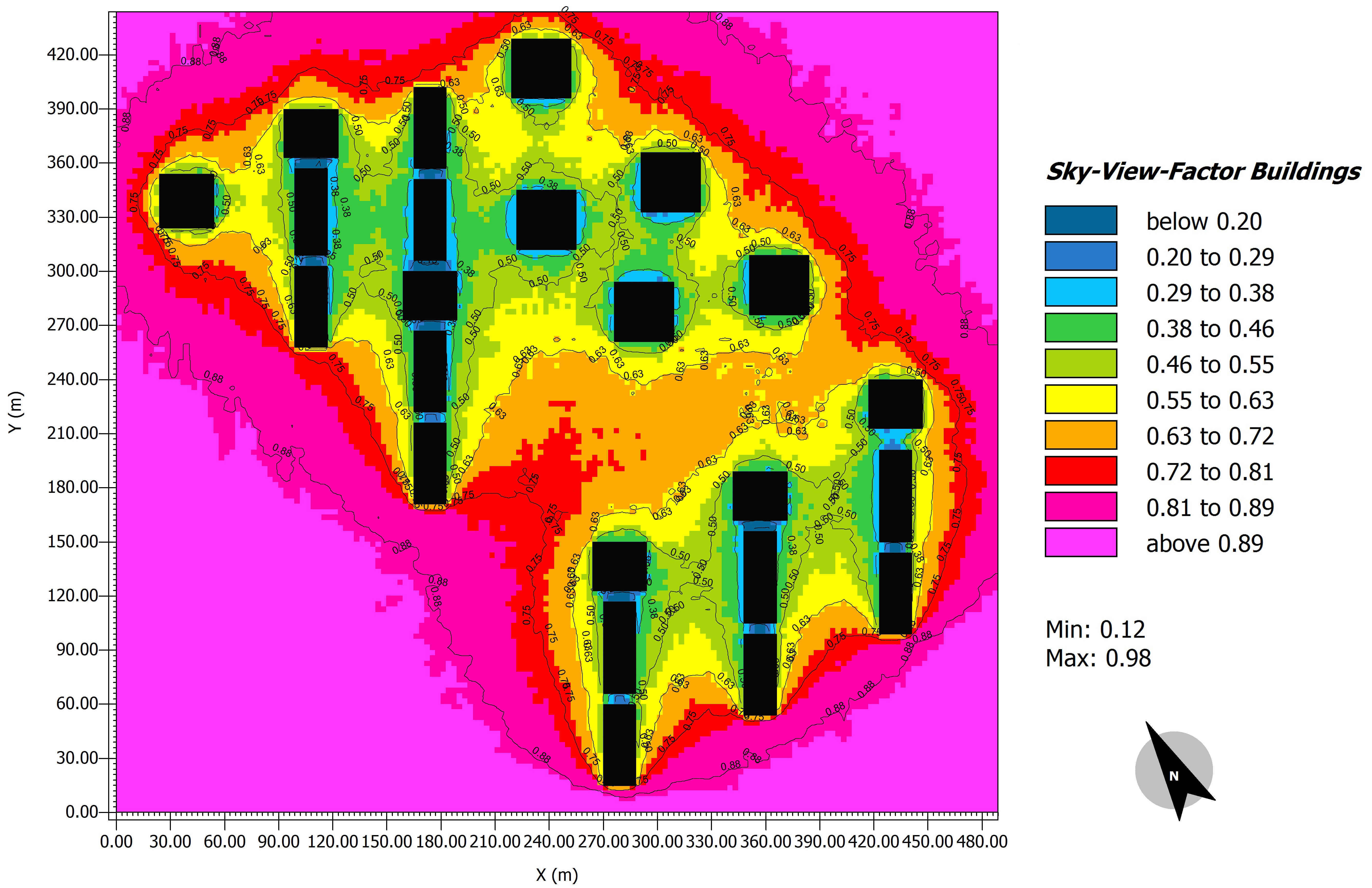
Fig. 5. The simulated SVF plan in the Atisaz residential complex.

Figure 6

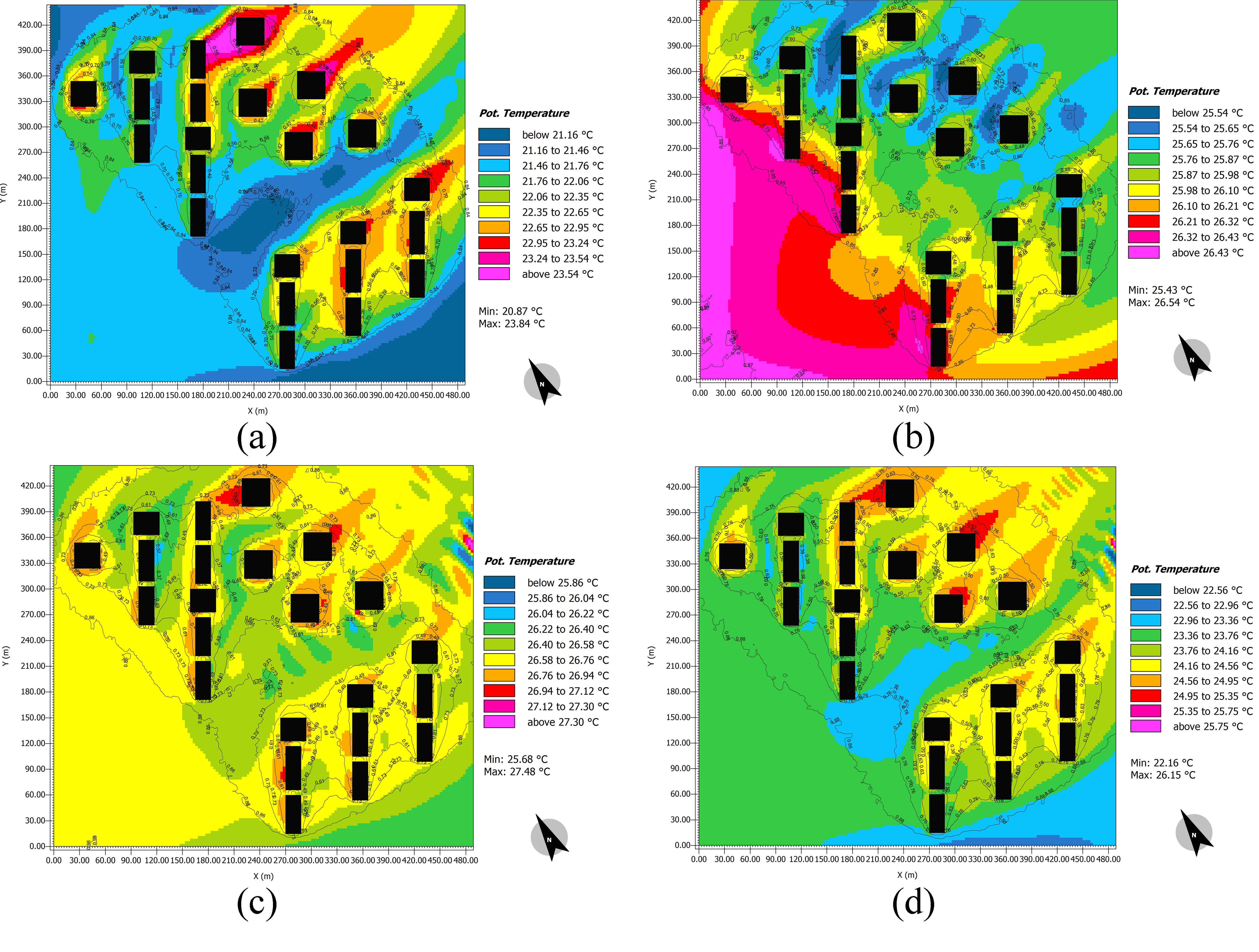
Fig. 6. The ENVI-met simulated air temperature plans at different hours (a) 5:00, (b) 11:00, (c) 17:00, and (d) 23:00 of the hottest day of the year.

Figure 7

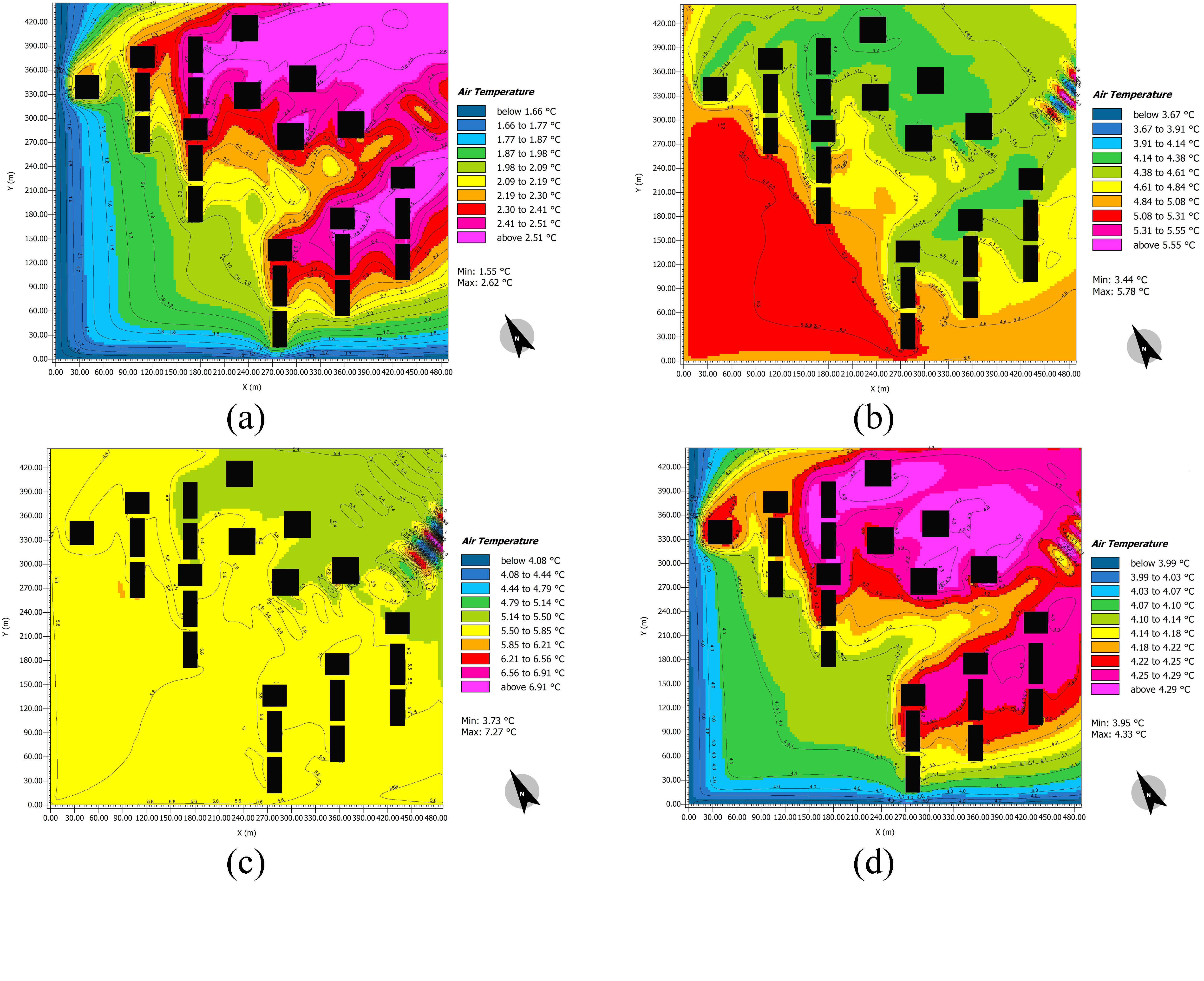
Fig. 7. The ENVI-met simulated air temperature plans at different hours of the coldest day of the year.

In the presence of solar radiation based on the thermal maps, the air temperature was determined to be lower than the surrounding environment in closed spaces where the SVF rate was low; however, when solar radiation is absent and its wavelength is not long enough to propagate into the space, especially before sunrise and after sunset, the inside air temperature was higher than the outer air temperature. The wind flow effects must be taken into consideration. When the surrounding outer space experiences a lower air temperature, in contrast, the wind shelters have a higher air temperature.

4. Results analysis using SPSS statistical software

The SPSS performs two scientific tests— a variance analysis and a regression analysis— on the results to clarify and to determine a correlation between air temperature and SVF during each hour of the hottest and coldest days of the year.

4.1. Validation of ENVI-met

An F test can be used to analyze the relationship between air temperature and SVF. To do so, the SVF factor can be classified into four categories [30].

Open space: 0.75 < SVF < 1
Semi-open space: 0.50 < SVF < 0.75
Semi-dense space: 0.25 < SVF < 0.50
Dense space: 0.00 < SVF < 0.25

Rather than considering all the air temperatures at all parts of the site, the average air temperature was considered in each of the SVF groups and these averages were compared. The air temperature was related to the SVF groups if the averages were significantly different. Thus, the dependent variable was air temperature, and the independent variable was the SVF factor, which was classified into four categories. According to Fig. 8, the data distribution is close to normal, so the conditions for using this test are reliable. Figure 8 illustrates a sample and the frequency at 5:00 am on the coldest day of the year.

Figure 8

Fig. 8. Frequency diagram of data distribution at 5:00 on the coldest day of the year.

By performing an F test for the hottest and coldest days of the year, the value of the Sig factor was achieved 0.00, which means that with a certainty of more than 99%, it can be said that there is a considerable difference among the average of the air temperature of the four categories.

In the next step, a Scheffe test was applied in which SVF groups were compared two by two. Table 3 shows the results of this test for all the hours of the hottest day and the coldest day of the year, and according to the value of Sig, the relation among each of these four groups at each time interval can be observed. For example, at all the hours of both hot and cold days of the year, the average air temperature and SVF in groups 3 and 4, i.e., semi-dense and dense groups, did not have a meaningful difference. In other cases, the value of Sig was less than 0.05, so it can be deduced that there was a meaningful difference among the groups.

Table 3

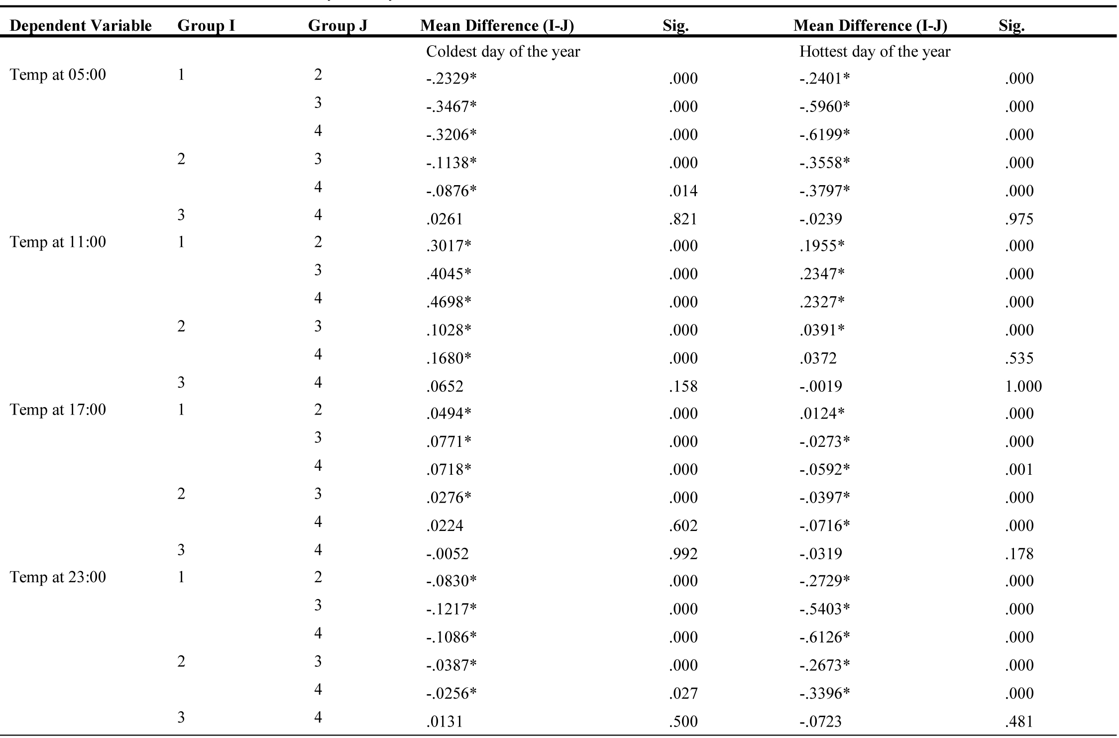
Table 3. Scheffe test of the hottest and coldest days of the year.

Figure 9 show the average air temperature in relation to the hours of the coldest and hottest days for four SVF groups. As can be observed, the relation between the air temperature of the weather and SVF at some hours was direct, and at other hours, the reverse was true. At some hours, there was no meaningful relation between the two factors.

Figure 9

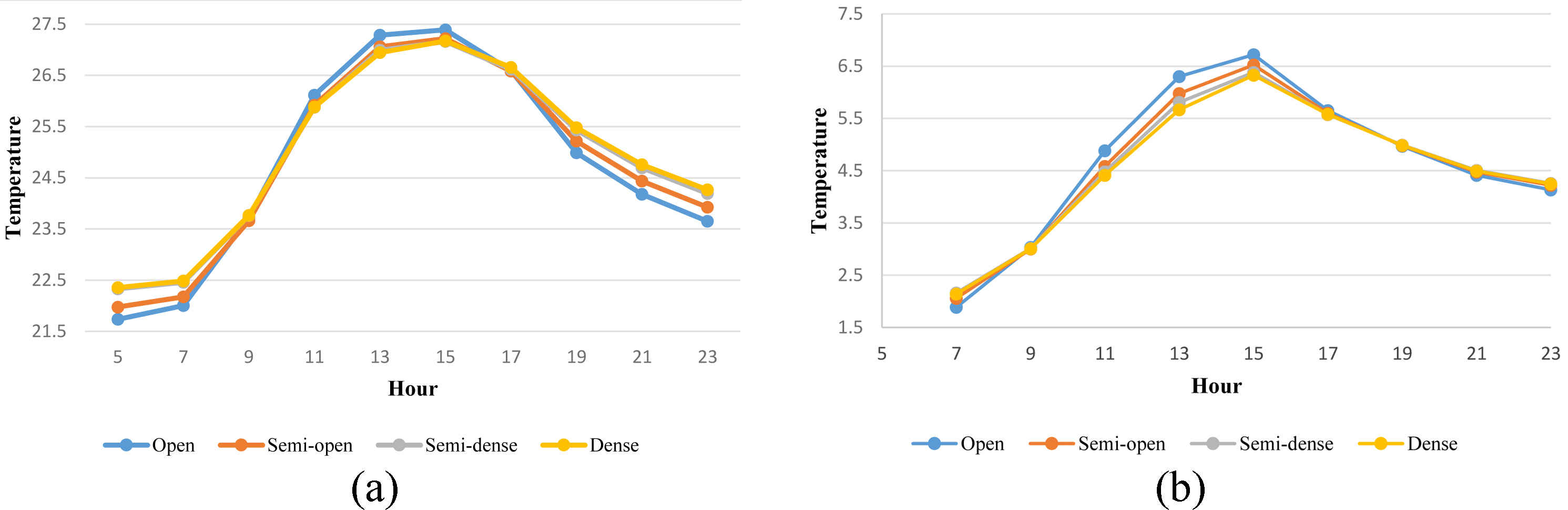
Fig. 9. The average air temperature in relation to the hours on the (a) hottest day and (b) coldest day for four SVF groups.

4.2. Regression analysis

In this step, and to determine the mathematical relation between the air temperature at different places of the site and the SVF factor, a regression analysis was performed. According to Table 4, the relation between the SVF factor and air temperature, such as at 5:00 a.m. on the coldest day of the year, was achieved as follow:

\[ T = -0.88×SVF+2.82 \]

Table 4

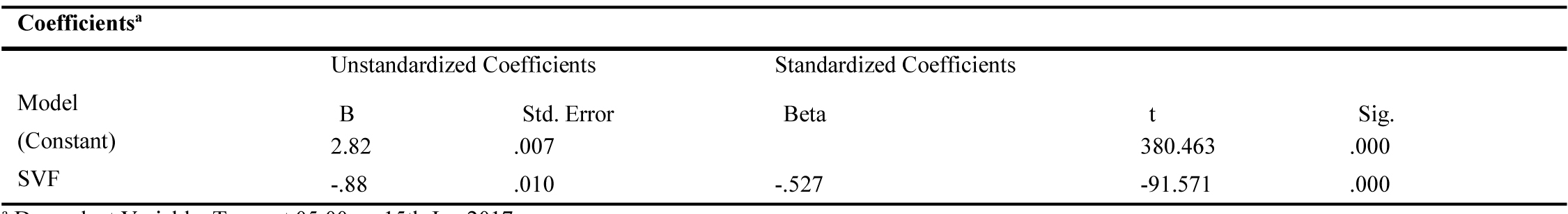
Table 4. A correlation between SVF and air temperature and coefficients.

In Table 5, the regression function (equation of a line between SVF and air temperature) was used for all the hours of the day on the coldest and hottest days. As can be observed, the negative or positive gradients of the lines in the regression diagrams show the direct and reverse relationship of air temperature and the SVF factor.

Table 5

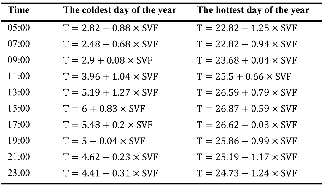
Table 5. Relationship of air temperature and SVF on the hottest and coldest days of the year.

When the gradient was positive, i.e., at 9, 11, 13, and 15 on the hottest day and at 9, 11, 13, 15, and 17 on the coldest day, the air temperature increased if SVF increased. When the gradient was negative, i.e., at 5, 7, 17, 19, 21, and 23 on the hottest day and at 5, 7, 19, 21, and 23 on the coldest day, the air temperature decreased if SVF increased.

5. Conclusions

This study investigated the relationship between SVF and variations in air temperature in an urban residential microclimate. Using a case study of an urban residential complex, details have been modeled in the ENVI-met model. The correlation of air temperature and SVF were analyzed using the statistical software of SPSS and by conducting two tests— a variance analysis and a regression analysis— for this scientific paper.

The obtained results from these tests and the graphs using ENVI-met show that before the warm hours such as at 5 am, 7 am, and after the warm hours, including 5 pm, 7 pm, 9 pm, and 11 pm, the correlation between SVF and air temperature was negative. In other words, as the SVF decreased, the air temperature increased subsequently; however, the air temperature rises because the SVF value is low in closed spaces and the heat is trapped between the buildings and cannot be emitted as a long wavelength into the outer spaces. There was a positive correlation between SVF and air temperature during the warm hours of the day, including 11 am, 1 pm, and 3 pm. In other words, as the SVF increased, the air temperature also increased. It can be concluded that in open spaces where the SVF is high, the higher the air temperature observed, whereas in closed spaces with a low SVF, the shadow diminishes the air temperature. There was a weak correlation between SVF and air temperature at 9 am. Hence, over all, for a well-balanced air temperature during the day and night, it is essential to optimize the air temperature with respect to SVF.

Another finding is that the results strongly indicate an air temperature difference of about 2–7°C between the residential site and its surrounding rural environment on the hottest day as well as 1-4°C on the coldest day. In addition, there was no noticeable difference in air temperature for dense and semi-dense spaces in the residential complex. Therefore, the geometry of a residential complex plays a decisive role in urban heat island mitigation. Moreover, SVF is suitable to be incorporated into residential urban design evaluations and decision making due to its potential key role as a geometry parameter of urban design.

To validate the obtained results of this scientific paper, it is suggested to analyze the data using a fish-eye photograph and a thermometer to measure the values of SVF and air temperature at different points because the results of this research are solely based on analytical software. In addition, further studies should be conducted, such as to evaluate the effect of vegetation on SVF and surface temperature. Eventually, by using the obtained data, this method can be used for different forms of buildings to achieve optimized urban forms.

Contributions

N. Nasrollahi conceived the study. G. Baghaeipoor collected data, performed simulations, interpreted the results, and wrote the manuscript. N. Nasrollahi supervised with help each stage of the project in terms of data collection, analysis and interpretation the analyses. N. Nasrollahi discussed the results and provided constructive advice to shape the project.

References

J. Zhang, C. K. Heng, L. C. Malone-Lee, D. Jun Chung Hii, P. Janssen, K. S. Leung, B.K. Tan, Evaluating environmental implications of density: A comparative case study on the relationship between density, urban block typology and sky exposure, Automation in Construction 22 (2012) 90-101. https://doi.org/10.1016/j.autcon.2011.06.011
M. P. J. Aarts, J. C. Stapel, T. A. M. C. Schoutens, J. van Hoof, Exploring the Impact of Natural Light Exposure on Sleep of Healthy Older Adults: A Field Study, Journal of Daylighting 5 (2018) 5-14. http://dx.doi.org/10.15627/jd.2018.2
S. M. Hosseini, M. Mohammadi, A. Rosemann, T. Schröder, Quantitative Investigation Through Climate-based Daylight Metrics of Visual Comfort Due to Colorful Glass and Orosi Windows in Iranian Architecture, Journal of Daylighting 5 (2018) 21-33. https://doi.org/10.15627/jd.2018.5
T. R. Oke, Canyon geometry and the nocturnal urban heat island: comparison of scale model and field observations, Journal of Climatology 1 (1981) 237-254. https://doi.org/10.1002/joc.3370010304
G. T. Johnson, I. D. Watson, The determination of view-factors in urban canyons, Journal of Climate and Applied Meteorology (1984) 329-335. https://doi.org/10.1175/1520-0450(1984)023%3C0329:tdovfi%3E2.0.co;2
J. M. Chen, T. A. BLACK, Measuring leaf area index of plant canopies with branch architecture, Agricultural and Forest Meteorology 57 (1991) 1–12. https://doi.org/10.1016/0168-1923(91)90074-z
P. Littlefair, Daylight, sunlight and solar gain in the urban environment, Solar Energy 70 (2001) 177–185. https://doi.org/10.1016/s0038-092x(00)00099-2
M.C. Anderson, Studies of the woodland light climate: I. The photographic computation of light conditions, Journal of Ecology 52 (1964) 27–41. https://doi.org/10.2307/2257780
D.G. Steyn, The calculation of view factors from fisheye-lens photographs: research note, Atmosphere-Ocean 18 (1980) 254-258. https://doi.org/10.1080/07055900.1980.9649091
L. Barring, J.O. Mattsson, S. Lindqvist, Canyon geometry, street temperatures and urban heat island in Malmö, Sweden, Journal of Climatology 5 (1985) 433-444. https://doi.org/10.1002/joc.3370050410
D.G. Steyn, I.D. Hay, I.D. Watson, G.T. Johnson, The determination of sky view factors in urban environments using video imagery, Journal of Atmospheric and Oceanic Technology3 (1986) 759-746. https://doi.org/10.1175/1520-0426(1986)003%3C0759:tdosvf%3E2.0.co;2
I. Eliasson, Infrared thermography and urban temperature patterns, Remote Sensing 13 (1992) 869-879. https://doi.org/10.1080/01431169208904160
U. PostgaÊrd, Road climate variation related to weather & topography, Ph.D. thesis, A52GU2000, Department of Physical Geography, University of Goteborg, Sweden, 2000. https://doi.org/10.1016%2Fj.egypro.2015.11.657
L. Chapman, J.E. Thornes, A.V. Bradley, Sky-view factor approximation using GPS receivers, International Journal of Climatology 22 (2002) 615–621. https://doi.org/10.1002/joc.649
L. Chapman, J.E. Thornes, Real-time sky-view factor calculation and approximation, Journal of Atmospheric and Oceanic Technology (2004) 730-742. https://doi.org/10.1175/1520-0426(2004)021%3C0730:rsfcaa%3E2.0.co;2
T.R. Oke, Boundary Layer Climates, Taylor & Francis e-Library, 1987.
C.Ratti, P. Richens, Urban texture analysis with image processing techniques, Paper presented at CAAD Futures 99, 1999, Atlanta, GA.
L. Chen, E. Ng, X. An, C. Ren, M. Lee, U.Wang, Z. He, Sky view factor analysis of street canyons and its implications for daytime intra-urban air temperature differentials in high-rise, high-density urban areas of Hong Kong: a GIS-based simulation approach, International Journal of Climatology 32 (2012) 121-136. https://doi.org/10.1002/joc.2243
T. Gál, F. Lindberg, J. Unger, Computing continuous sky view factors using 3D urban raster and vector databases: comparison and application to urban climate, Theoretical and Applied Climatology 95 (2009) 111-123. https://doi.org/10.1007/s00704-007-0362-9
J. Bernard, E. Bocher, G. Petit, S. Palominos, Sky View Factor Calculation in Urban Context: Computational Performance and Accuracy Analysis of Two Open and Free GIS Tools, Special Issue "Urban Overheating - Progress on Mitigation Science and Engineering Applications", Climate, 6 (2018) 60-84. https://doi.org/10.3390/cli6030060
J. Liang, J. Gong, J. Sun, J. Liu, A customizable framework for computing sky view factor from large-scale 3D city models, Energy and Buildings 149 (2017) 38-44. https://doi.org/10.1016/j.enbuild.2017.05.024
S. Mirzaee, O. Özgun, M. Ruth, K. C. Binita, Neighborhood-scale sky view factor variations with building density and height: A simulation approach and case study of Boston, Urban climate 26 (2018) 95-108. https://doi.org/10.1016/j.uclim.2018.08.012
T. Gál, J. Unger, A new software tool for SVF calculations using building and tree-crown databases, Urban Climate 10 (2014) 594-606. https://doi.org/10.1016/j.uclim.2014.05.004
J. Ramírez-Faz, R. Lopez-Luque, F.J. Casares, Development of synthetic hemispheric projections suitable for assessing the sky view factor on vertical planes, Renewable Energy 74 (2015) 279-286. https://doi.org/10.1016/j.renene.2014.08.025
J. Rakovec, K. Zaksek, On the proper analytical expression for the sky-view factor and the diffuse irradiation of a slope for an isotropic sky, Renewable Energy 37 (2012) 440-444. https://doi.org/10.1016/j.renene.2011.06.042
T.R. Oke, G.T. Johnson, D.G. Steyn, I.D. Watson, Simulation of surface urban heat islands under ‘ideal’ conditions at night. Part 2: diagnosis of causation, Boundary-Layer Meteorology 56 (1991) 339-358. https://doi.org/10.1007/bf00119211
I. Eliasson, Urban nocturnal temperatures, street geometry and land use, Atmospheric Environment 30 (1996) 379-392. https://doi.org/10.1016/1352-2310(95)00033-x
S. Yamashita, K. Sekine, M. Shoda, K. Yamashita, Y. Hara, On relationships between heat island and sky view factor in the cities of Tama river basin, Japan, Atmospheric Environment 20 (1986) 681–686. https://doi.org/10.1016/0004-6981(86)90182-4
I.M. Karlsson, Nocturnal air temperature variations between forest and open areas, Journal of Applied Meteorology 39 (2000) 851– 862. https://doi.org/10.1175/1520-0450(2000)039%3C0851:natvbf%3E2.0.co;2
M.K. Svensson, Sky view factor analysis-implications for urban air temperature differences, Meteorological Applications 11 (2004) 201-211. https://doi.org/10.1017/s1350482704001288
J. Unger, Intra-urban relationship between surface geometry and urban heat island: review and new approach, Climate Research 27 (2004) 253-264. https://doi.org/10.3354/cr027253
X. Yang, Y. Li,The impact of building density and building height heterogeneity on average urban albedo and street surface temperature, Building and Environment 90 (2015) 146-156. https://doi.org/10.1016/j.buildenv.2015.03.037
B.W. Atkinson, Numerical modelling of urban heat-island intensity, Boundary-Layer Meteorology 109 (2003) 285–310. https://doi.org/10.1023/a:1025820326672
K. Steemers, M. Ramos, M. Sinou, Urban diversity. In Environmental Diversity in Architecture, K. Steemers, M.A. Steane eds., Spon Press, London, New York, 2004.
S. Blankenstein, W. Kuttler, Impact of street geometry on downward longwave radiation and air temperature in an urban environment, Meteorologische Zeitschrift 13 (2004) 373- 379. https://doi.org/10.1127/0941-2948/2004/0013-0373
F. Bourbia, F. Boucheriba, Impact of street design on urban microclimate for semi-arid climate (Constantine), Renew Energy 35 (2010) 343-347. https://doi.org/10.1016/j.renene.2009.07.017
F. Bourbia, H.B. Awbi, Building cluster and shading in urban canyon for hot dry climate: part 1: air and surface temperature measurements, Renew Energy 29 (2004) 249-262. https://doi.org/10.1016/s0960-1481(03)00170-8
R. Giridharan, S. Ganesan, S.S.Y. Lau, Daytime urban heat island effect in high-rise high-density developments in Hong Kong, Energy and Buildings 36 (2004) 525–534. https://doi.org/10.1016/j.enbuild.2003.12.016
R. Giridharan, S.S. Y Lau, S.Ganesan, B. Givoni, Urban design factors influencing heat island intensity in high-rise high-density environments of Hong Kong, Building and Environment 42 (2007) 3669–3684. https://doi.org/10.1016/j.buildenv.2006.09.011
F. Bourbia, H.B. Awbi, Building cluster and shading in urban canyon for hot dry climate part 2, shading simulations, Renew Energy 29 (2004) 291-301. https://doi.org/10.1016/s0960-1481(03)00171-x
F. Lindberg, I. Eliasson, B. Holmer, Urban geometry and temperature variations, 5th Int. Conf. on urban climate, 2003.
H. Upmanis, D. Chen, Influence of geographical factors and meteorological variables on nocturnal urban-park temperature differences - a case study of summer 1995 in Goteborg, Sweden, Climate Research 13 (1999) 125-139. https://doi.org/10.3354/cr013125
atisazco.ir, retrieved: 21/07/2018
https://earth.google.com/web, retrieved: 21/07/2018.
Envi-met simulation software, http://www.envi-met.com/#section/intro, retrieved by 21/07/2018.
Y. Toparlar, B. Blocken, B. Maiheu, G.J.F. van Heijst, A review on the CFD analysis of urban microclimate, Renewable and Sustainable Energy Reviews 80 (2017)1613-1640. https://doi.org/10.1016/j.rser.2017.05.248
M. Bruse, H. Fleer, Simulating surface–plant–air interactions inside urban environments with a three dimensional numerical model, Environmental Modelling & Software 13 (1998) 373-384. https://doi.org/10.1016/s1364-8152(98)00042-5
S. Tsoka, A.Tsikaloudaki, T.Theodosiou, Analyzing the ENVI-met microclimate model’s performance and assessing cool materials and urban vegetation applications-a review, Sustainable cities and society 43 (2018) 55-76. https://doi.org/10.1016/j.scs.2018.08.009
N. Nasrollahi, Z. Hatami, M. Taleghani, Development of outdoor thermal comfort model for tourists in urban historical areas; A case study in Isfahan, Building and Environment 125 (2017) 356-372. https://doi.org/10.1016/j.buildenv.2017.09.006
M. Taleghani, L. Kleerekoper, M.Tenpierik, A. van den Dobbelsteen, Outdoor thermal comfort within five different urban forms in the Netherlands, Building and Environment 83 (2015) 65-78. https://doi.org/10.1016/j.buildenv.2014.03.014
Y. Wang, H. Akbari, Analysis of urban heat island phenomenon and mitigation solutions evaluation for Montreal, Sustainable Cities and Society 26 (2016) 438–446. https://doi.org/10.1016/j.scs.2016.04.015
http://irimo.ir/eng/wd/720-Products-Services.html, retrieved: 01/06/2018.

Get PDF (16 MB)

SHARE ON