Volume 7 Issue 1 > pp. 1-12 • doi: 10.15627/jd.2020.1
Outdoor Investigation of High Concentrator Photovoltaic Under Uniform and Non-Uniform Illumination
Hashem Shatnawi,* Abdulrahman Aldossary
Author affiliations
Jubail Technical Institute, PO Box 10335, Jubail Industrial City 31961, Saudi Arabia
* Corresponding author. Tel. +96613-3402641; Fax: +96613-3418722
hashem121@yahoo.com (H. Shatnawi)
aldossary@hotmail.co.uk (A. Aldossary)
History: Received 28 November 2019 | Revised 9 January 2020 | Accepted 20 January 2020 | Published online 13 February 2020
Copyright: © 2020 The Author(s). Published by solarlits.com. This is an open access article under the CC BY license (http://creativecommons.org/licenses/by/4.0/).
Citation: Hashem Shatnawi, Abdulrahman Aldossary, Outdoor Investigation of High Concentrator Photovoltaic Under Uniform and Non-Uniform Illumination, Journal of Daylighting 7 (2020) 1-12. http://dx.doi.org/10.15627/jd.2020.1
Figures and tables
Abstract
This study was performed in outdoor conditions to quantify the level of influence on the electrical performance of the Multi-junction (MJ) solar cells. It was discovered that non-uniform illumination on the solar cell could reduce the MJ electrical output by more than 40%. Also, the irradiation uniformity was improved by applying several methods; increasing the distance between the concentrator and the receiver (l) and introducing a secondary optical element (SOE) on the receiver. The outdoor measurement also revealed that the electrical efficiency of the solar cell increased from around 22% to 37% with an increment of 68%, due to improvement of irradiation uniformity. However, the optical efficiency substantially fell when increasing the distance (l). To address this issue, a 0.06 m high SOE having a surface reflectivity of 90% above the PV assembly was implemented to enhance the irradiation uniformity and to minimise the dramatic decline in optical efficiency. The hot spot initiated by non-uniform illumination was also examined in outdoor conditions by measuring the temperature at the centre and both sides of the PV cell. Accordingly, a variance of about 13 K was observed between the centre and both sides (0.005 m distance) of the PV cell’s surface area, which was further reduced to 1 K after improving the illumination uniformity.
Keywords
Multi-junction solar cells, Non-uniform illumination, Electrical efficiency, Fresnel lens
1. Introduction
Multi-junction (MJ) solar cells nowadays are more favoured compared to single-junction cells in integrating into high concentrator PV (HCPV) systems since they are more efficient, with improved response to the high concentration and a lower temperature coefficient. Utilising new technology in the generation of III-V MJ solar cells offers higher efficiencies that exceed 43% at high concentrations compared to conventional solar cells made of a single layer of semiconductor material [1]. Semiconductor compounds such as Gallium Arsenide from group III and V of the periodic table, offer the highest PV conversion efficiency [2-5]. MJ solar cells comprise of a stack of layered p-n junctions each made from a different set of semiconductors having a different band gap and spectral absorption in order to capture as much of the solar spectrum as feasible. Semiconductors in a triple-junction solar cell such as Ge, GaInAs/GaAs and GaInP are most commonly used given their high optical absorption coefficients and adequate values of minority carrier lifetimes and mobilities [2,6,7].
In a triple-junction solar cell the first layer (GaInP) converts the short wavelength portion of the spectrum, the second layer (GaInAs) captures the near-infrared light and the third layer (Ge) absorbs the lower photon energies of the infrared radiation. Henry [8] calculated the terrestrial MJ solar cell restrictive theoretical conversion efficiency under 1000 sun concentrations with the solar cell maintained at room temperature with 1, 2, 3 and 36 band gaps in which the corresponding efficiencies were 37, 50, 56 and 72%. Thus, this technology can be considered as the most promising among the other PV technologies.
On the other hand, the primary challenge of using an MJ solar cell is related to the initial development and operational costs in generating electricity if compared to power generated from conventional sources. Different techniques have previously been investigated and introduced to improve the efficiency of solar power generation in order to become more affordable (cost-effective) such as applying a Concentrator PV (CPV) using an optical concentrator such as a Fresnel lens [9-11], parabolic troughs [12], dishes [13], and a compound parabolic concentrator [14] in reducing energy generation costs [15]. CPV systems replace the expensive semiconductor PV material with inexpensive material such as glass, mirrors and plastic to concentrate a large area of sunlight onto a smaller area of the solar cell. CPV is characterised into three groups based on the amount of solar concentration; low (LCPV), medium (MCPV) and high concentration (HCPV).
Nowadays, Fresnel lenses are the preferred choice since they have numerous advantages when compared to other concentrators given their small volume, light-weight, able to be mass-produced at a relatively low cost and efficiently increase energy density [9]. However, the Fresnel lens produces high non-uniform illumination and temperature on the PV cell, causing hot spots, current mismatch and reduces the overall efficiency of the system [15]. Additionally, the distribution of received flux on the PV cell is a key issue especially at high concentration ratios as PV cells require uniform flux in gaining optimum performance [10,16,17].
Non-uniformity can form over a single surface area of the solar cell or a series of connected cells. In the first case, there is excessive illumination on some areas of the solar cells, while for other areas, the cells are rarely illuminated. The illuminated areas excessively produce high currents and become overly heated, which decreases the electrical output of the solar cell. In contrast, some areas of the solar cell fail to operate with the generation of cross-currents causing dissipation of electrical power [15]. In the second case where the solar cells are connected in series, the generated current and performance of the cells is restricted to the cells having the worst distribution of illumination or having the least illumination [18].
In the case of MJ solar cells, high non-uniformity increases the amount of power loss (I2R) in the high concentration areas causing the cells to become less efficient in generating power [19]. Vishnoi et al. [20] described the combined effect of non-uniform illumination and surface resistance on the performance of the solar cell. The researchers found that the dark regions in a partially illuminated cell act as a load responsible for the decline in conversion efficiency, open-circuit voltage (VOC) and short circuit current (ISC) values. Whereas Franklin and Coventry, [16] investigated the effects of non-uniformity on the I–V curve parameters of the MJ solar cell by comparing two solar cells under uniform and non-uniform illumination . The findings indicated that the ‘fill factor’ (FF) value (the ratio of maximum power (Pm) from the solar cell to the theoretical power (PT)) of a solar cell under non-uniform illumination was much lower. In another study by Herrero et al. [10], they analysed the effect of non-uniformity on MJ cells and discovered that the FF decreased with an increase in non-uniformity. Here, they contributed this decline to the increase in a series of resistance losses, thereby reducing the efficiency of the solar cell. In a separate study, Araki and Yamaguchi [21] modelled the interaction between the chromatic aberration and non-uniform flux distribution and simulated the effect on both performance and efficiency of the solar cell. In this case, the fill factor was anticipated to improve given the presence of chromatic aberration at the expense of a low short circuit current (Isc). However, the results indicated that the recovery of FF by chromatic aberration was not sufficient enough to counter the damage caused by non-uniform illumination
A secondary optical element (SOE), acknowledged as a more traditional method, is often used to improve the illumination homogeneity on the surface of the receiver [11,15,22] and is considered appropriate to use with reflective or refractive CPV systems. These elements (SOEs) are commonly integrated into HCPV systems, typically point-focus Fresnel lenses in which the concentration ratios exceed 100 suns [23]. Regarding SOEs, there are a variety of different types such as refractive, reflective or both. For example, V-trough, refractive CPCs, refractive silos and hollow inverted pyramid reflectors [23,24]. Reflective SOEs are less expensive and are reasonably easier to produce compared to refractive ones. However, the only disadvantage of integrating SOEs into such systems is that by increasing the number of optical components in the optical system, the optical efficiency may subsequently be reduced [25].
Even though integrating a point-focus Fresnel lens and MJ solar cell in HCPV systems is seen as an emerging technology, limited studies describe the performance of the system under uniform and non-uniform illumination, particularly with respect to outdoor environments under real ambient conditions. Moreover, the majority of studies tend to depict the effect of non-uniform illumination using a qualitative approach, whereas, in this study, a quantitative approach is adopted to examine the optical and electrical performance of a single HCPV system installed outdoors. Two techniques are employed to increase the uniformity on the receiver (PV cell). First, by increasing the distance between the Fresnel lens and the PV cell from the focus point, and secondly, by introducing a SOE on the receiver. The primary objective of this experiment is to acquire uniform irradiation on the receiver with nominal loss in the energy received, (i.e. minimum loss in optical efficiency as compared to the energy received at the focus point without a SOE). In achieving this objective, the extent of non-uniformity will be examined via visual inspection, temperature distribution on the solar cell and its effect on the electrical performance and efficiency of the HCPV system.
2. Outdoor experimental setup
The purpose of this study is to quantify the negative influence of the non-uniform illumination and the hot spot on the HCPV electrical performance under real ambient conditions. Therefore, the testing experimental setup including the HCPV system, supporting fixtures and data acquisition system were assembled outdoor. The HCPV system consists of the following main components: optical elements, solar cell, and cooling mechanism as shown in Fig. 1.
Figure 1
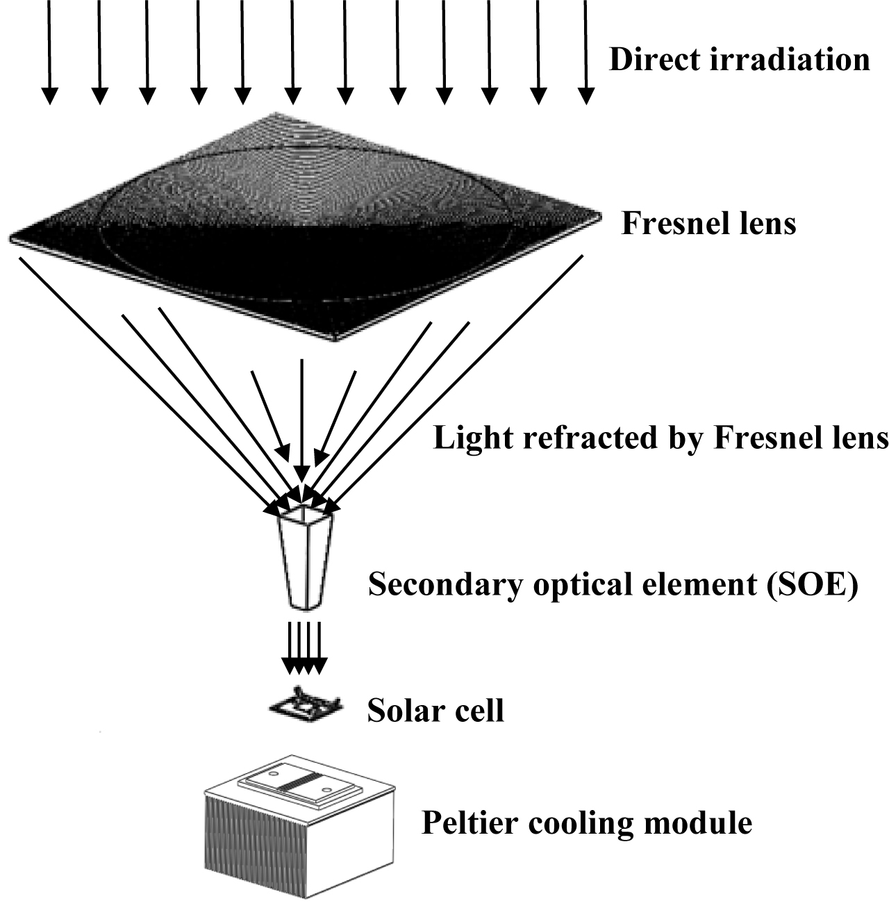
Fig. 1. HCPV system principle and exploded view of its components.
2.1. HCPV system
2.1.1. HCPV system
There are two optical elements in this HCPV system, point-focus Fresnel lens as a primary optical element (POE) and hollow inverted truncated pyramid reflector (HITPR) as a SOE. The Fresnel lens parameters including the focal length (f), thickness and transmissivity are listed in Table 1. The active size of the Fresnel lens (aperture (a)) and the PV cell (receiver (r)) are 0.0625 m2 and 0.0001 m2 respectively. Hence, the resulted geometrical concentration ratio (GCR) is 625X which is the maximum concentration ratio (CR) that can be achieved if no optical losses occurred. However, this GCR can be controlled by controlling the Fresnel lens aperture area exposed to the sun light. For example, if the needed GCR is 100X then the aperture area of 0.1x0.1 m2 can only be exposed to the sun light and the rest can be covered.
where GCR is the geometrical concentration ratio, Aa is the area of the aperture (Fresnel lens), Ar is the area of the receiver (PV), ηopt is the optical efficiency of the Fresnel lens, and CR is the Concentration Ratio.
Table 1
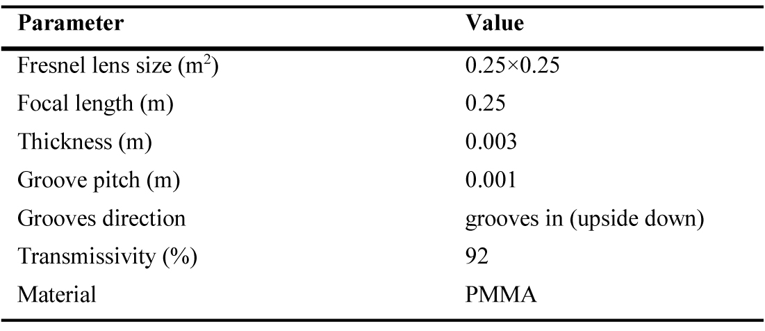
Table 1. Designing parameters of the Fresnel lens.
The SOE was designed using SolidWorks; a schematic diagram of the developed SOE with its geometrical dimensions is shown in Fig. 2.
Figure 2
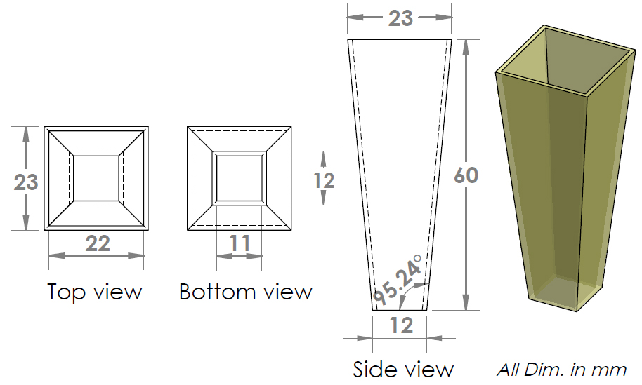
Fig. 2. Schematic diagram of the developed SOE.
The exit aperture area of the SOE (0.011×0.011 m2) was chosen based on the PV cell area (0.01×0.01 m2) with 0.0005 m margin from each side and the area of the entrance aperture (0.000484 m2) is four times the exit aperture area (0.000121 m2) to collect the highest amount of refracted rays. The SOE was made by a 3D printer using a transparent FullCure 720 rigid material [26]. After making the SOE, the four inner walls were covered by four pieces of high reflective material with overall average reflectivity of 90% [27] using 3M double face tape as shown in Fig. 3.
Figure 3
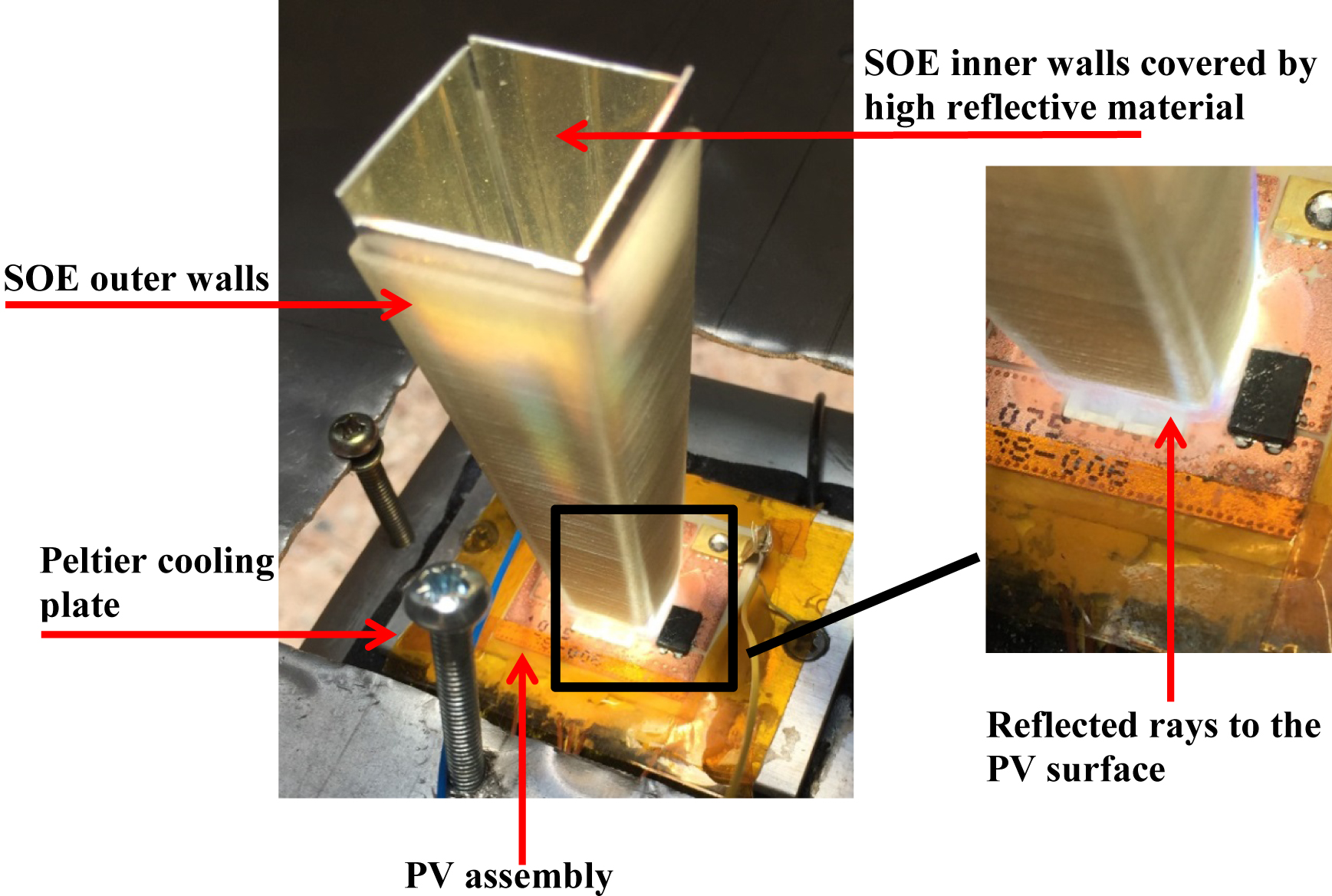
Fig. 3. SOE inner walls covered by high reflective material.
2.1.2. Multi-junction solar cell
High efficiency triple-junction (TJ) PV assembly made of GaInP-GaInAs-Ge and area of 0.0316×0.0296 m2with active surface of 0.0001 m2 was integrated to the HCPV system. The typical electrical conversion efficiency of this solar cell obtained at standard controlled lab steady conditions is about 40% under the following measurement settings: 500X (X = 1000 W/m2), PV cell temperature of 25oC, air mass (AM) of 1.5, solar spectral irradiance of ASTM G173-03 and uniform direct irradiance [28].
2.1.3. Cooling system
A 12V Peltier cooling module with rated power of 60 W and area of 0.04×0.04 m2 powered by a DC power supply was used to cool the PV cell. To measure the PV average temperature experimentally and assess the hot spot produced by the non-uniform ray distribution, three T- type surface thermocouples were attached at the back of the solar cell surface using Aluminium Foil tape and their tips were fully covered from the surrounding air Fig. 4(a). The three thermocouples located at the centre, right and left side (i.e. 0.005 m spacing distance) under the PV active surface Fig. 4(b). Three U-shaped grooves on the Peltier cooling module Aluminium plate with dimensions of 0.0015×0.00075 m2 were made to accommodate the three 0.00013 m diameter thermocouples underneath the PV and to ensure that the PV assembly is in full contact with the cooling module. The bottom side of the solar cell assembly was attached to a the Peltier module using high conductivity thermal paste (3 W/m∙K) [29].
Figure 4
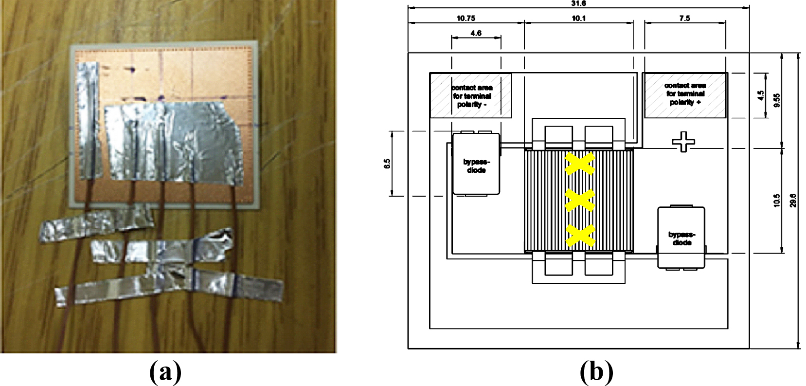
Fig. 4. (a) Thermocouples attached at the back of the solar cell assembly and (b) their locations (letter X).
2.2. Supporting fixtures
The HCPV housing was fabricated from light weight weather resistant 0.0007 m Aluminium sheet to support and firmly fit the Fresnel lens wooden frame as shown in Fig. 5. The dimensions of the HCPV housing were chosen based on the Fresnel lens size and its focal length which are 0.25×0.25×0.25 m3. Also, a housing base with dimensions 0.26×0.26 m2 was fabricated from 0.0007 m Aluminium sheet and 0.01 m from each side of the housing base was bended up to attach the HCPV housing firmly on a 1x1x0.02 m3 flat surface wooden plate using four screws. A 0.07×0.07 m2square hole was made in the housing base and wooden plate to accommodate the Peltier cooling module where the PV assembly is attached. The wooden plate was securely screwed to an adjustable angle plate where the whole assembly can be tilted at the required angle. The adjustable angle plate which carries the whole assembly is also securely screwed on a workshop wheel trolley for easy movement.
Figure 5
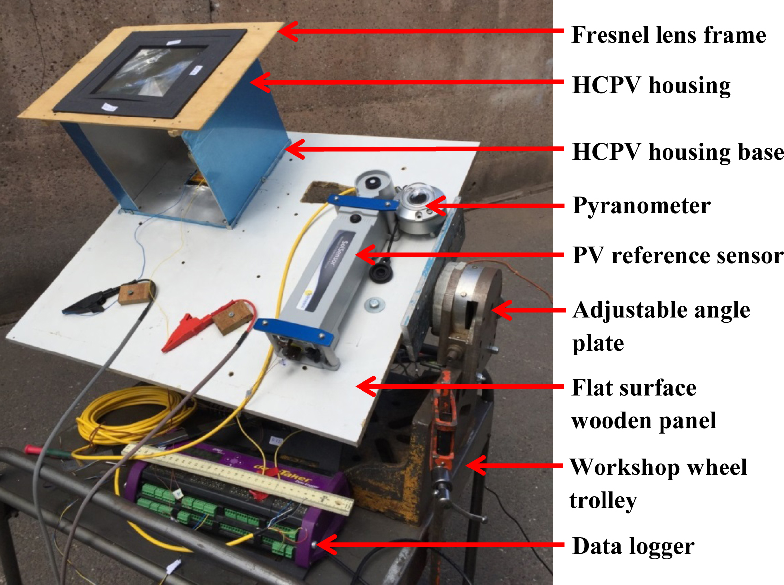
Fig. 5. Workshop wheel trolley carries the whole HCPV assembly.
2.3. Data acquisition system
Figure 6 shows a schematic diagram of the test rig including the measuring devices. Solmetric PV analyser kit (PVA-1000S) [30] was used to characterise the HCPV outdoor. This kit includes two main units: I-V curve tracer and wireless PV reference sensor. The I-V curve tracer is able to produce an instant I-V and P-V curves for the solar cell and measure the following electrical parameters: VOC, ISC, current at maximum power (Im), voltage at maximum power (Vm), Pm and FF. Simultaneously, the wireless PV reference sensor unit measures the following parameters: PV cell and ambient temperature, solar irradiance at the aperture and tilt angle of the system. The measurement duration including the I-V curve sweep is only 4 seconds. The solar irradiance measurements using wireless PV reference sensor were confirmed by a new certified and calibrated Kipp & Zonen SMP10 Pyranometer [31].
Figure 6
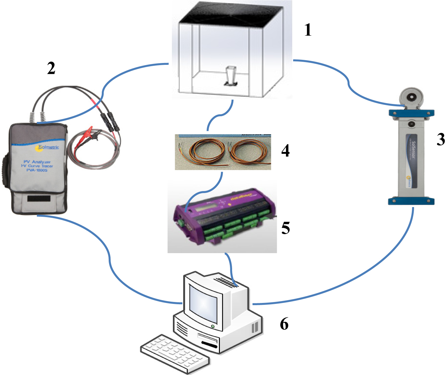
Fig. 6. The test rig with the instrumentations. 1: HCPV system, 2: I-V curve tracer, 3: PV reference sensor, 4: Thermocouples, 5: Data logger, and 6: Data processor.
Table 2 summarises the specifications of the above two measuring units i.e. I-V curve tracer and wireless PV reference sensor including the measurement range, resolution and accuracy of the measured parameters.
Table 2
![Specifications of the I-V curve tracer and wireless PV reference sensor [32].](figures/7-1-20.jpg)
Table 2. Specifications of the I-V curve tracer and wireless PV reference sensor [32].
3. Outdoor experimental procedure
The outdoor experiment was carried out between September 2018 and April 2019 for optical and electrical characterisation. The test facility was completed when all the parts were assembled and all measuring devices were connected. All the measuring data was collected at reference temperature of the PV cell i.e. 25 °C. Before any data collection, the adjustable angle plate was set to zero i.e. in horizontal position and a spirit level was placed at different locations on the Fresnel lens top surface to confirm that the whole assembly is properly aligned. Due to the movement of the sun, the adjustable angle plate and workshop wheel trolley were used to point the HCPV system toward the sun position during the data collection. A shadow stick was placed on the reference surface where the HCPV was seated to confirm that the assembly is normal to sun light by observing the shadow direction and length where no shadow indicate that the assembly is normal to the sunlight [33].
3.1. Optical characterisation
The developed HCPV was examined outdoor in terms of optical efficiency (ηopt) and incident illumination uniformity with and without SOE. For optical efficiency calculation, the ratio of the average irradiation power on the receiver to the average irradiation power on the aperture can be determined through Eq. (3).
where ηopt is the optical efficiency, Pr is the average irradiation power on the receiver, and Pa is the average irradiation power on the aperture.
To measure the average solar flux on the aperture, the wireless PV reference sensor was used. While, the ISCwas measured using the I-V curve tracer to determine the average irradiation power on the receiver [34,35].
3.2. Electrical characterisation
The developed HCPV system was electrically examined outdoor under different concentration ratios by varying the Fresnel lens aperture area exposed to the sun light. The PV temperature was controlled by controlling the input power to the Peltier cooling module by a variable DC power supply. Also, the electrical performance of the TJ solar cell was examined under different incident illumination profile such as point-focus and more uniform illumination to evaluate its influence. Electrical efficiency (ηelect) can be defined as the ratio of the Pm generated by the solar cell to the average irradiation power on the receiver Pr equation (4). The Pm (equation (5)) was measured directly by the I-V tracer and Pr (equation (6)) was calculated from the measured ISC.
where ηelect is the electrical efficiency, Pm is the maximum power generated by the solar cell, Pr is the average irradiation power on the receiver, Im is the current at maximum power, Vm is the voltage at maximum power Ir is the average irradiance on the receiver, and Ar is the area of the receiver (PV).
4. Results and discussions
4.1. HCPV performance without SOE
Five different Fresnel lens aperture areas 0.13×0.13, 0.15×0.15, 0.18×0.18, 0.2×0.2 and 0.25×0.25 m2 with the following geometrical concentration ratios were examined experimentally to determine their optical efficiency at the focus point (f = l = 0.25 m) without SOE: 169X, 225X, 324X, 400X and 625X. Figure 7 shows the experimental optical efficiency results. The optical efficiency decreased from about 72% at geometrical concentration ratio of 169X to about 55% at geometrical concentration ratio of 625X with more than 20% drop. It is clear from this figure that the optical loses increase when the geometrical concentration ratio increase leading to a lower optical efficiency. The depth of the Fresnel lens prism and slope angle (α) increase with the distance from the centre axis of the Fresnel lens. Therefore, higher GCR (bigger aperture area) results in higher number of deeper prisms that experience more reflection losses and material absorption than shallow ones [36].
Figure 7
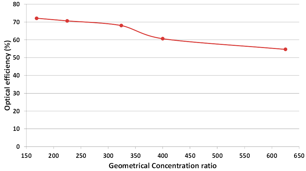
Fig. 7. Experimental optical efficiency.
Figure 8 shows the experimental illumination profile on the solar cell when the TJ solar cell was placed underneath the Fresnel lens with aperture area of 0.18×0.18 m2 at its focus point i.e. at distance f = 0.25m. The point-focus profile is clear on the PV surface.
Figure 8
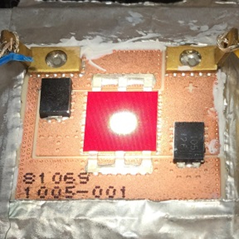
Fig. 8. Experimental incident rays profile.
Figure 9 shows the 2D temperature distribution including the centre and sides temperature of the solar cell for the Fresnel lens with aperture areas of 0.13×0.13 m2, 0.18×0.18 m2 and 0.25×0.25 m2. As shown in the Figure, the temperature at the centre of the PV in all tested Fresnel lens apertures was higher than the sides and the temperature difference was dependent on the concentration ratio. As the aperture area increases, the non-uniform illumination on the solar cell increases causing higher gradient in temperature between the centre and the sides of the cell. For example, the centre temperature of the 0.25×0.25 m2 aperture area Fresnel lens was 17°C higher than the two sides while in case of 0.13×0.13 m2 the difference was less than 5°C.
Figure 9
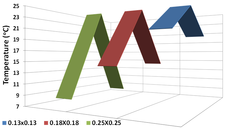
Fig. 9. 2D measured temperature distribution of the solar cell for different Fresnel lens aperture areas.
The influence of varying the distance (l) on the optical and electrical performances of the HCPV and received irradiance uniformity for 0.18x0.18m2 Fresnel lens aperture area was examined experimentally. The distance (l) was increased from 0.250-0.295 m with a step of 0.005 m. Figure 10 shows that the optical efficiency is negatively influenced by increasing the distance (l). The converged received radiation flux on the solar cell become more diverge as distance (l) increases which leads to a loss of partial radiation flux received by the solar cell. It can be seen that the experimental optical efficiency drops from about 63% at focus point i.e. f = l = 0.25 m to about 12% at l=0.295 m.
Figure 10
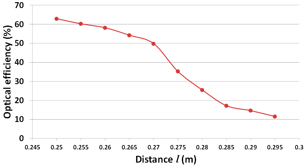
Fig. 10. Experimental optical efficiency at different distance of (l).
Figure 11 shows the effect of increasing the distance (l) on both experimental optical and electrical efficiency. As the distance (l) increases the electrical efficiency increases; this may refer to the improvement in the incident illumination uniformity. The electrical efficiency increased from about 22% at focus point to about 37% at l=0.295 m with increase of about 68%. In other words, non-uniform illumination on the solar cell can reduce the MJ electrical output by more than 40%.
Figure 11
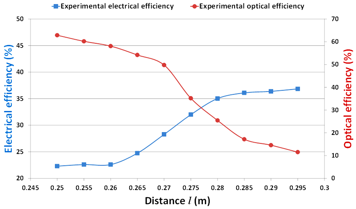
Fig. 11. Experimental optical and electrical efficiency of HCPV with distance (l).
Figure 12 shows the 2D measured temperature distribution underneath the PV for the 0.18×0.18 m2 aperture area Fresnel lens at focus point and at l=0.295 m. At l=0.295 m the temperature difference is very small (about 1 oC) while at point-focus illumination the temperature difference is about 13 oC. The hot spot is almost eliminated by increasing the incident rays uniformity.
Figure 12
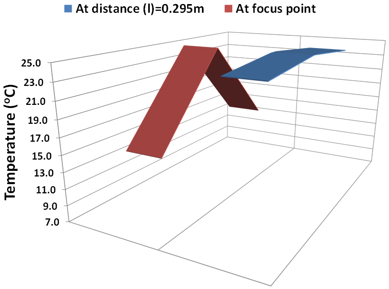
Fig. 12. 2D PV measured temperature distribution at focus point and at l=0.295 m.
Figure 13 shows a summary of the testing results including the experimental electrical efficiency and received radiation flux profile as the distance (l) increases for the Fresnel lens with aperture area of 0.18×0.18 m2. Although the electrical efficiency was improved due to the better incident rays distribution on the solar cell, the optical efficiency was dropped from about 63% at focus point to about 15% at l=0.29 m (Fig. 10). It is crucial to maintain the optical efficiency while improving the incident rays uniformity. Although the optical efficiency at l=0.25 m is the highest, the electrical efficiency is the lowest where the non-uniform illumination and temperature at this height is maximum. As discussed in the introduction part, non-uniform illumination and temperature on the solar cell cause hot spot and current mismatches leading to a reduction in the overall electrical efficiency of the system.
Figure 13
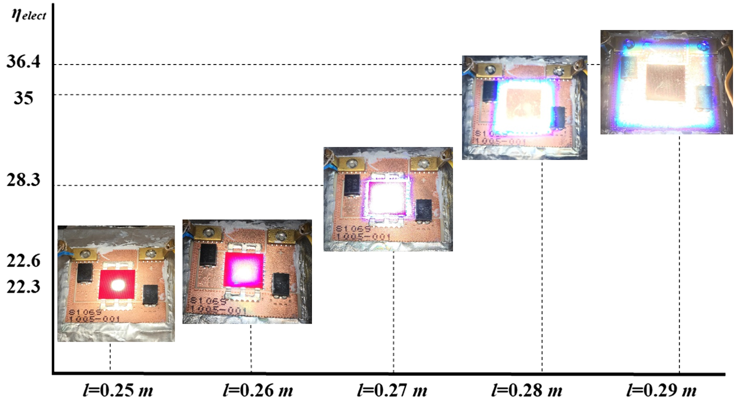
Fig. 13. Experimental electrical efficiency and received flux distribution at different values of (l), without SOE.
4.2. HCPV performance with SOE
Figure 14 shows the experimental optical efficiency of the HCPV after introducing the 0.06 m SOE. Unlike the optical efficiency descending trend when increasing the distance (l) without SOE, with SOE the optical efficiency increases as the distance (l) increased. This can be referred to the increase in the total acceptance angle of the optical system as the distance (l) increases which allow more rays to enter the SOE aperture and reflected to the solar cell.
Figure 14
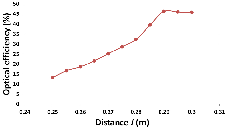
Fig. 14. Experimental optical efficiency of the lens at different distance of (l) with SOE.
Figure 15 shows the experimental electrical and optical efficiencies of the HCPV after incorporating the SOE. For both optical and electrical parameters, efficiencies increase till reaching the optimum distance at l=0.29 m where after this point the curve starts descending. At l=0.29 m, the electrical and optical efficiencies are the highest. The optical experimental efficiency increased from about 13% at the focus point to more than 46% at l=0.29 m while the electrical efficiency increased from about 28% to about 36%. Unlike the case where there is no SOE, the incident radiation flux on the solar cell is more uniform which makes the effect of non-uniform illumination on the electrical output less significant. Therefore, the maximum electrical efficiency matches the maximum optical efficiency point i.e. at l=0.29 m.
Figure 15
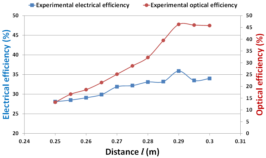
Fig. 15. Experimental optical and electrical efficiencies of the HCPV at different distance of (l) with SOE.
Table 3 shows a summary of the testing results including the electrical efficiency and optical efficiency for the Fresnel lens with aperture area of 0.18×0.18m2 at focus point (l=0.25 m), at l=0.29 m and at l= 0.29 m with integrating 0.06m SOE. The experimental optical efficiency increased more than 200% after placing the SOE compared to the case at the same distance (l) but without SOE. It increased from about 15% to 45% with maintaining almost the same electrical efficiency i.e. 36.4% compared to 35.9%. Therefore, a combination of placing a SOE and increasing distance (l) is better than only increasing the distance (l) to improve the irradiation uniformity and enhance the HCPV performance.
Table 3
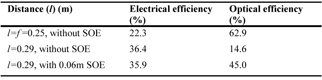
Table 3. Summary of optical and electrical examinations with and without SOE.
The optical losses increase by increasing the number of the optical elements in a CPV system which can be observed from the Table above where the total optical efficiency reduced from about 63% to 45% after introducing the SOE with reduction of about 29%. But, the gain in the electrical efficiency after improving the incident flux uniformity using the SOE is more than 60% which can compensate this loss. To increase the optical efficiency of the optical system a higher reflective material for the SOE can be used. Also, a parametric study of the Fresnel lens to optimise the optical performance can be done in a separate study.
Figures 16 and 17 show the outdoor experimental I-V and power curves for the solar cell under CR= 119X and 74X at reference temperature with and without SOE. It can be seen that VOC and the maximum power Pm increased after increasing the irradiation uniformity by introducing the SOE.
Table 4 summarises the influence of introducing the developed SOE on VOC and Pm for the above two concentration ratios 119X and 74X. This Table shows that placing the SOE at concentration ratio of 119X would increase the output electrical power and efficiency by about 14%. Moreover, at lower concentration ratio i.e. 74X where the negative influence of degree of non-uniformity is less, the electrical power and efficiency was increased by about 8%.
Table 4

Table 4. Summary of optical and electrical examinations with and without SOE.
Figure 16
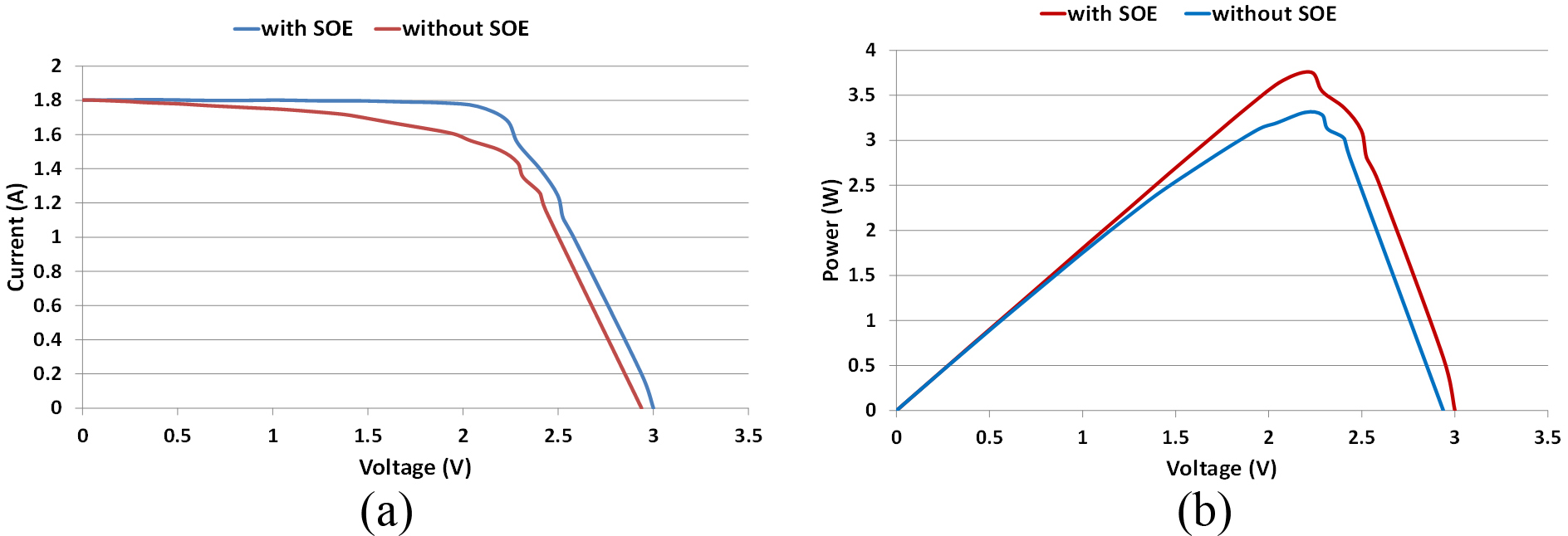
Fig. 16. (a) Outdoor I-V curves and (b) power curves at CR=119X and PV temperature of 25°C.
Figure 17
Fig. 17. (a) Outdoor I-V curves and (b) power curves at CR=74X and PV temperature of 25°C.
4.3. Measurements accuracy
All surface thermocouples used in the experiment were calibrated using RTD Pt100 with high accuracy of ±0.025 K and the uncertainties in their measurement can be calculated using Root Square Sum (RSS) of the systematic and random errors [32]
where Ust is uncertainty of the standard (RTD), Ucurve-fit is the uncertainty of the curve fit and Uthermo is the overall uncertainty of the thermocouple sensors.
The curve fit error is statistical and can be calculated as [32]
where tn-1,95% is the student distribution factor for degree of freedom n -1 and n is the number of sample data.
Sx̄ is the standard deviation of the mean given by
σ is the standard deviation which can be calculated using:
where xi is the RTD reading, x̄ is the curve fit value and Xi-x̄2 is the deviation squared. Table 5 shows the calculation of the uncertainty for one of the surface thermocouples.
Table 5
Table 5. Surface thermocouple measurement uncertainty calculations.
The standard device used in the calibration is high precision RTD which was calibrated against ice temperature i.e. at 0 oC as it was placed in the ice water mixture and the temperature was recorded at different points as shown in Fig. 18. The uncertainty of the RTD Pt100 sensor (Ust) is small i.e. ±0.025K compared to the uncertainty of the measuring device (Ucurve-fit). Therefore, the overall uncertainty of the surface thermocouple sensors calculated using equation 3.4 is ±0.20K.
Figure 18
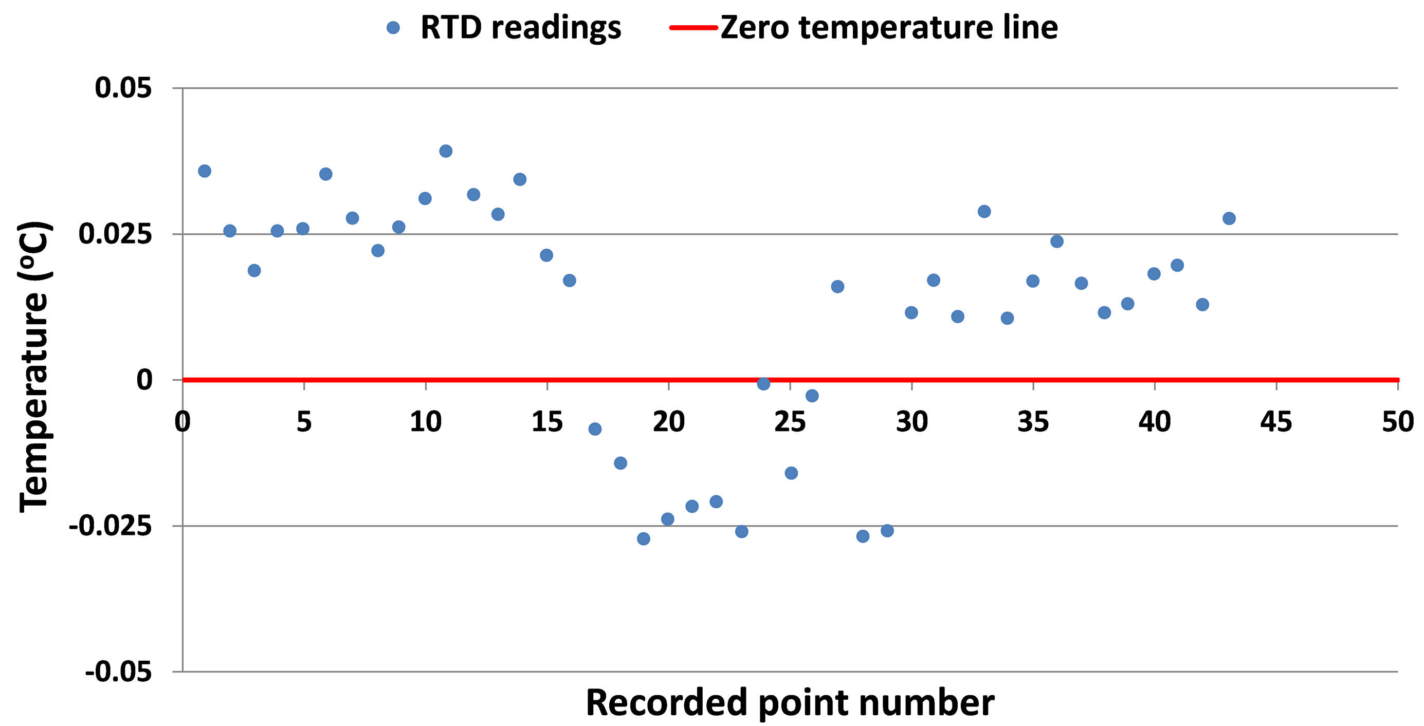
Fig. 18. Calibration of the RTD thermocouple reading.
The wireless PV reference sensor is used to measure the solar radiation at the aperture of the Fresnel lens. It was calibrated against a certified new Kipp & Zonen SMP10 Pyranometer. The uncertainty of the irradiance PV reference sensor (Uirr) is then calculated based on the uncertainty of the curve fitting (Ucurve-fit) and uncertainty of the Pyranometer (Upyr) as shown in Eq. (11) [32].
The uncertainty of the Pyranometer is given by the manufacturer in the calibration certificate (Upyr) to be ±0.76 W/m2 and the uncertainty of the measuring device (Ucurve-fit) is 2.44 W/m2 as shown in Table 6. Therefore, the overall uncertainty of the radiation sensor calculated using equation 11 is ±2.56 W/m2.
Table 6
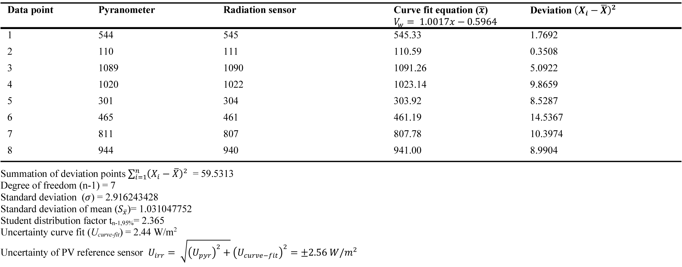
Table 6. Radiation measurement at the aperture uncertainty calculations.
5. Conclusions
The influence of non-uniform illumination and the hot spot on the electrical efficiency of the MJ solar cell in this study was analysed quantitatively and examined outdoor under real ambient conditions. Outdoor examination revealed that non-uniform illumination on the solar cell can reduce the MJ electrical output by more than 40%.
The irradiation uniformity was improved by increasing the distance between the concentrator and the receiver (l) to spread the illumination over the PV assembly. The electrical efficiency of the solar cell has increased from about 22% to about 37% with an increment of 68% after improving the irradiation uniformity by increasing the distance (l) to 0.295 m. However, the optical efficiency has dropped substantially.
Therefore, a 0.06 m high secondary optical element (SOE) with surface reflectivity of 90% above the PV assembly was introduced to increase the irradiation uniformity as well as minimise the sever drop in the optical efficiency. The optical efficiency increased more than 200% after placing the SOE compared to the case at the same distance (l) but without SOE. It increased from about 15% to 45% with maintaining almost the same electrical efficiency i.e. 36.4% compared to 35.9%. Therefore, a combination of placing a SOE and increasing distance (l) is better than only increasing the distance (l) to improve the irradiation uniformity and enhance the HCPV performance.
The hot spot initiated by the non-uniform illumination was assessed experimentally by measuring the centre and sides surface temperatures of the PV under 0.18x0.18 m2Fresnel lens. At focus point i.e. l= 0.25 m, a difference of about 13 K was found between the centre and the side (0.005 m distance) of the PV surface; but after using the designed SOE to improve the illumination uniformity a difference of about 1 K was measured.
The effect of non-uniform incident rays on the solar cell I-V and power curves were investigated. It was clear that the negative influence of non-uniform illumination is more at higher concentration ratios. The maximum power (Pm) improved after placing the SOE due to the improvement in the open circuit voltage (VOC) with electrical efficiency increment of about 14% and 8% at CR = 119X and 74X respectively.
It will be useful if the experimental outputs in this study is used as a reference to develop optical and electrical mathematical models for optimisation purpose, which can be undertaken in a separate study.
Contributions
The authors have contributed equally.
References
- L. Micheli, N. Sarmah, X. Luo, K. Reddy, and T. Mallick, Opportunities and challenges in micro-and nano-technologies for concentrating photovoltaic cooling: A review, Renewable and Sustainable Energy Reviews 20 (2013) 595-610. https://doi.org/10.1016/j.rser.2012.11.051
- IRENA, Renewable energy technologies: Cost analysis series, International Renewable Energy Agency, 2012.
- I. S. E. Fraunhofer, New world record for solar cell efficiency at 46%, Available online: https://www.ise.fraunhofer.de/en/press-and-media/press-releases/press-releases-2014/new-world-record-for-solar-cell-efficiency-at-46-percent, accessed on: 1 November, 2019.
- E. Wesoff, Sharp Hits Record 44.4% Efficiency for Triple-Junction Solar Cell , Available online: http://www.greentechmedia.com/articles/read/Sharp-Hits-Record-44.4-Efficiency-For-Triple-Junction-Solar-Cell, accessed on 1 Nov 2019.
- R. King, D. Law, K. Edmondson, C. Fetzer, G. Kinsey, H. Yoon, R. Sherif , N. Karam, 40% efficient metamorphic GaInP∕ GaInAs∕ Ge multijunction solar cells, Applied physics letters 90 (2007) 183516. https://doi.org/10.1063/1.2734507
- J. Olson, D. Friedman, and S. Kurtz, High-efficiency III-V multijunction solar cells, in Handbook of Photovoltaic Science and Engineering, John Wiley & Sons, Ltd, UK, 2003. https://doi.org/10.1002/9780470974704.ch8
- R. Miles, K. Hynes, and I. Forbes, Photovoltaic solar cells: An overview of state-of-the-art cell development and environmental issues, Progress in Crystal Growth and Characterization of Materials 51 (2005) 1-42. https://doi.org/10.1016/j.pcrysgrow.2005.10.002
- C. Henry, Limiting efficiencies of ideal single and multiple energy gap terrestrial solar cells, Journal of applied physics 51 (1980) 4494-4500. https://doi.org/10.1063/1.328272
- W. Xie, Y. Dai, R. Wang, and K. Sumathy, Concentrated solar energy applications using Fresnel lenses: A review, Renewable and Sustainable Energy Reviews 15 (2011) 2588-2606. https://doi.org/10.1016/j.rser.2011.03.031
- R. Herrero, M. Victoria, C. Domínguez, S. Askins, I. Antón, and G. Sala, Concentration photovoltaic optical system irradiance distribution measurements and its effect on multi‐junction solar cells, Progress in Photovoltaics: Research and Applications 20 (2012) 423-430. https://doi.org/10.1002/pip.1145
- P. Benítez, JC. Miñano, P. Zamora, R. Mohedano, A. Cvetkovic, M. Buljan, J. Chaves, M. Hernández, High performance Fresnel-based photovoltaic concentrator, Optics express 18 (2010) A25-A40. https://doi.org/10.1364/oe.18.000a25
- D. Krüger, Y. Pandian, K. Hennecke, and M. Schmitz, Parabolic trough collector testing in the frame of the REACt project, Desalination 220 (2008) 612-618. https://doi.org/10.1016/j.desal.2007.04.062
- T. Tao, H. Zheng, Y. Su, and S. Riffat, A novel combined solar concentration/wind augmentation system: Constructions and preliminary testing of a prototype, Applied Thermal Engineering 31 (2011) 3664-3668. https://doi.org/10.1016/j.applthermaleng.2011.01.015
- T. Mallick and P. Eames, Design and fabrication of low concentrating second generation PRIDE concentrator, Solar Energy Materials and Solar Cells 91 (2007) 597-608. https://doi.org/10.1016/j.solmat.2006.11.016
- H. Baig, K. Heasman, and T. Mallick, Non-uniform illumination in concentrating solar cells, Renewable and Sustainable Energy Reviews 16 (2012) 5890-5909. https://doi.org/10.1016/j.rser.2012.06.020
- E. Franklin and J. Coventry, Effects of highly non-uniform illumination distribution on electrical performance of solar cells, in: Proceedings of Solar 2002, 2002, Boulder, Colo, American Solar Energy Society.
- E. Katz, J. Gordon, and D. Feuermann, Effects of ultra‐high flux and intensity distribution in multi‐junction solar cells, Progress in Photovoltaics: Research and Applications 14 (2006) 297-303. https://doi.org/10.1002/pip.670
- J. Coventry, Performance of a concentrating photovoltaic/thermal solar collector, Solar energy 78 (2005) 211-222. https://doi.org/10.1016/j.solener.2004.03.014
- R. D. Nasby and R. W. Sanderson, Performance measurement techniques for concentrator photovoltaic cells, Solar Cells 6 (1982) 39-47. https://doi.org/10.1016/0379-6787(82)90016-3 [
- A. VISHNOI, R. Ggopal, R. Dwivedi, and S. K. Srivastava, Combined effect of non-uniform illumination and surface resistance on the performance of a solar cell, International Journal of Electronics 66 (1989) 755-774. https://doi.org/10.1080/00207218908925431
- K. Araki and M. Yamaguchi, Extended distributed model for analysis of non-ideal concentration operation, Solar energy materials and solar cells 75 (2003) 467-473. https://doi.org/10.1016/s0927-0248(02)00203-9
- M. Victoria, R. Herrero, C. Domínguez, I. Antón, S. Askins, and G. Sala, Characterization of the spatial distribution of irradiance and spectrum in concentrating photovoltaic systems and their effect on multi‐junction solar cells, Progress in Photovoltaics: Research and Applications 21 (2013) 308-318. https://doi.org/10.1002/pip.1183
- R. Swanson, Photovoltaic concentrators, Handbook of photovoltaic science and engineering, 2003, pp. 449-503, John Wiley & Sons, Ltd. https://doi.org/10.1002/9780470974704
- M. Buljan, J. Mendes, P. Benítez, and J. Miñano, Recent trends in concentrated photovoltaics concentrators’ architecture, Journal of Photonics for Energy 4 (2014) 040995. https://doi.org/10.1117/1.jpe.4.040995
- V. Andreev, V. Grilikhes, V. Khvostikov, O. Khvostikova, V. Rumyantsev, N. Sadchikov, M. Shvarts M, Concentrator PV modules and solar cells for TPV systems, Solar energy materials and solar cells 84 (2004) 3-17. https://doi.org/10.1016/j.solmat.2004.02.037
- BuildParts - Materials - FullCure 720, Available online: http://www.buildparts.com/materials/fullcure720, accessed on: 10 Nov, 2019.
- Technical information of alanod solar relective material, Alanod-Solar, Available online: https://www.alanod.com/products, accessed on: 10 Nov 2019.
- AZURSPACE, Enhanced Fresnel Assembly Concentrating Photovoltaic (CPV) Modules, Available online: http://www.azurspace.com/images/products/DB_3987-00-00_3C42_AzurDesign_EFA_10x10_2014-03-27.pdf, accessed on 11 Nov, 2019.
- HTSP Silicone Heat Transfer Compound Plus, Available online: http://www.electrolube.com/core/components/products/tds/044/HTSP.pdf, accessed on: 11 Nov, 2019.
- PVA-1000S PV Analyzer Kit Solmetric, Available online: http://www.solmetric.com/pvanalyzermatrix.html, accessed on: 11 Nov 2019.
- SMP10 pyranometer, the smartest way to measure solar radiation Kipp & Zonen, Available online: http://www.kippzonen.com/Product/281/SMP10-Pyranometer#.WCIVCS2LSpp, accessed on: 11 Nov 2019.
- A. Elsayed, Heat transfer in helically coiled small diameter tubes for miniature cooling systems, Diss. University of Birmingham, 2011.
- A. M. El-Nashar, Seasonal effect of dust deposition on a field of evacuated tube collectors on the performance of a solar desalination plant, Desalination 239 (2009) 66-81. https://doi.org/10.1016/j.desal.2008.03.007
- K.-K. Chong, S.-L. Lau, T.-K. Yew, P. Chee-Lin Tan, Design and development in optics of concentrator photovoltaic system, Renewable and Sustainable Energy Reviews 19 (2013) 598-612. https://doi.org/10.1016/j.rser.2012.11.005
- I. Wallhead, T. Jiménez, J. Ortiz, I. Toledo, C. Toledo, Design of an efficient Fresnel-type lens utilizing double total internal reflection for solar energy collection, Optics express 20 (2012) A1005-A1010. https://doi.org/10.1364/oe.20.0a1005
- L. Micheli, N. Sarmah, X. Luo, K. Reddy, and T. Mallick, Opportunities and challenges in micro-and nano-technologies for concentrating photovoltaic cooling: A review, Renewable and Sustainable Energy Reviews 20 (2013) 595-610. https://doi.org/10.1016/j.rser.2012.11.051
Copyright © 2020 The Author(s). Published by solarlits.com.

1979
Total views
Citations
SHARE ON


