The Impact of Courtyard and Street Canyon Surroundings on Global Illuminance and Estimated UV Index in the Tropics

^a Building Physics Research Group, Faculty of Industrial Technology, Institut Teknologi Bandung, Jl. Ganesha 10, Labtek VI, Bandung 40132, Indonesia
^b Building Technology Research Group, School of Architecture, Planning, and Policy Development, Institut Teknologi Bandung, Jl. Ganesha 10, Labtek VI, Bandung 40132, Indonesia
^c Architecture Program, Faculty of Technology and Vocational Education, Universitas Pendidikan Indonesia, Jl. Dr. Setiabudhi 229, Bandung 40152, Indonesia

* Corresponding author.
armanto@tf.itb.ac.id (R. A. Mangkuto)
donny@ar.itb.ac.id (M. D. Koerniawan)
betaparamita@upi.edu (B. Paramita)

History: Received 12 June 2020 | Revised 15 July 2020 | Accepted 30 July 2020 | Published online 24 August 2020

Citation: Rizki A. Mangkuto, Mochamad Donny Koerniawan, Beta Paramita, The Impact of Courtyard and Street Canyon Surroundings on Global Illuminance and Estimated UV Index in the Tropics, Journal of Daylighting 7 (2020) 167-185. https://dx.doi.org/10.15627/jd.2020.16

Figures and tables

Figure 1
Figure 2
Figure 3
Table 1
Table 2
Figure 4
Figure 5
Figure 6
Figure 7
Figure 8
Figure 9
Figure 10
Figure 11
Table 3
Table 4
Table 5
Figure 12
Figure 13
Table 6
Table 7
Table 8

Abstract

Exposing oneself to outdoor daylight in the morning can be healthy and harmful at the same time, due to the risk of ultraviolet exposure. The presence of surrounding buildings in the urban context may also influence the risk. This study aims to identify the impact of courtyard and street canyon surroundings of various size and heights on the peak time and values of global illuminances and ultraviolet index (UVI), for the case of a tropical city. The impact of the surroundings is estimated by performing annual daylighting simulation with Daysim, considering various receiving plane orientations, followed with sensitivity analysis. The results suggest that in the courtyard scenes, on 21 March, 21 June, and 22 December, the maximum horizontal UVI are respectively 9 at 12.00 hrs, 9 at 10.00 hrs, and 5 at 11.00 hrs, while the corresponding, maximum vertical UVI are 6, facing east at 09.00 hrs; 8, northeast at 10.00 hrs; and 3, southeast at 08.00 hrs. In the street canyon scenes, the 5m wide street is more sensitive to height variation, compared to the 10-m wide. The maximum horizontal UVI on the three days are 10, 9, and 5; while the corresponding, maximum vertical UVI are 6, east; 9, northeast; and 4, southeast; all with the same peak time as in the courtyard scenes. Sensitivity analysis results from the three days are found to be more reliable than those from the entire year. The study thus has the main contribution in providing the methodology in estimating UVI under various outdoor scenarios with surrounding buildings, particularly in the tropical region.

Keywords

Global illuminance, Ultraviolet index, Sensitivity analysis, Daylighting simulation

Nomenclature

d	order of day in the year [-]
d’	normalised order of day in the year [-]
E	east orientation
EAS	erythemal action spectrum [-]
E_e,g	global irradiance received on a surface [W/m²]
E_v,g	global illuminance received on a surface [lx]
H	hour mark
h	building blocks height [m]
h’	normalised building blocks height [-]
K_g	global luminous efficacy [lm/W]
m	minutes pass the hour mark
N	north orientation
NE	northeast orientation
NW	northwest orientation
R²	coefficient of determination [-]
R²_adj	adjusted coefficient of determination [-]
S	south orientation
SE	southeast orientation
SRC	standardised regression coefficient [-]
SW	southwest orientation
s	courtyard size [m]
s’	normalised courtyard size [-]
t	time stamp [hh.mm]
UVI	ultraviolet index [-]
UVI’	normalised ultraviolet index [-]
W	west orientation
w	street width [m]
w’	normalised street width [-]
α	street orientation [°]
α’	normalised street orientation [-]
β’	standardised regression coefficient [-]
ε	residual error [-]
λ	wavelength [nm]
μ_x	mean of input parameter
μ_y	mean of output parameter
σ_x	standard deviation of input parameter
σ_y	standard deviation of output parameter

1. Introduction

During the recent outbreak of the novel coronavirus disease (COVID-19), there are various popular information suggesting a number of ways for healthy people to maintain or increase the immunity of their body. One of the suggestions is to expose oneself to outdoor day- or sunlight (i.e. ‘sunbathing’) for a short period, particularly in the morning time. The ultraviolet (UV) radiation of the sunlight on one hand stimulates the production of vitamin D, which is important in maintaining healthful bones, and may help the body in suppressing the risk of development of various diseases such as cancer, diabetes, arthritis, and others [1-5]. While there is still no strong evidence on whether sunlight exposure is effective in lowering the risk of COVID-19 infection; on the other hand, it is clear that excessive and prolonged exposure of sunlight on human skin may lead to various harmful effects, such as sunburn, skin cancer, skin ageing, and many others [5,6].

Due to the conflicting nature of sunlight exposure on human, there have been discussions, particularly in the medical science, photochemistry and photobiology communities, on the optimum period and duration on healthy sunlight exposure. From the point of view of environmental science, the quantity of sunlight on any point on earth depends on the geographical location, time of day, and date, which altogether determine the solar elevation angle; as well as atmospheric and other relevant climate-related conditions; which eventually determine the amount of global, diffuse, and direct solar irradiance. However, solar irradiance and the eventual UV index (UVI) are typically measured in a horizontal plane, as per guidelines and common practices [7-9]. The measurement station is also often located in a place relatively free from nearby obstacles or surrounding buildings, such as in the vicinity of an airport. Consequently, the reported irradiance data, e.g. in the form of climate data, most probably represent the upper values for unobstructed exterior scenes.

In the current case where people wish to do expose themselves to outdoor daylight while self-isolating at home and minimising close contact with other people, it is highly not advisable to do so at an open, outdoor field. The feasible location would be then limited to a certain open area near or around the residential buildings. In the urban context, very often there are surrounding buildings that can significantly reduce the amount of solar irradiance, and thus also the UVI on that limited open area, due to the shading effect. The reduction may be attributed to several factors, which among others are the layout and size of the surrounding buildings (height, width) and of the open area itself, and the surface reflectance of the building surroundings. This study focuses on the first two factors, since both are related with the direct view towards the sky. The influence of reflectance is not systematically observed here, since it is considered less influential on the received light quantity in scenes with either daylighting [10,11] or electric lighting [12]. There are many possibilities of surrounding buildings layout, but for simplicity, two general layouts or scenes can be considered here: (1) a courtyard, which is a compact, open plane surrounded with four building blocks [13,14], and (2) a street canyon, which is an open plane whose length is significantly larger than its width, surrounded with two parallel building blocks of also considerable height [15,16].

The receiving planes in this case are also not always horizontal. While standing, one’s face and torso would be on a vertical plane, and thus orientation also has an important role. Since terrestrial global irradiance is space- and time-dependent, it may be of interest to determine the peak time of the values measured on horizontal and vertical planes on various days of the year, at a particular location with certain surrounding buildings. It is also important to understand how the surroundings affect the temporal daylight performance, and how they affects the estimated UVI at that location at any particular time.

The widely validated daylighting simulation program Daysim [17-20] is employed to estimate the global illuminance profile at the receiving planes of interest. Daysim is a Radiance-based program that works using standard EnergyPlus weather (EPW) data file as input, combined with the relevant building geometry. The output however typically only returns illuminance values, as it is mostly applied to predict indoor daylighting performance. Conversion to irradiance can nevertheless be made, since the program assumes the luminous efficacy and sky luminance distribution for the Perez all-weather sky model [19,21,22].

Having presented the relevant tools, the present study has therefore the following objectives: (1) to determine the impact of surrounding buildings, in this case courtyard and street canyon, on the global illuminance profile and the estimated UVI, by performing annual daylighting simulation; and (2) to identify the peak time of global horizontal and vertical illuminances and the estimated UVI at a particular location with certain surrounding buildings. The applied methods are described in Section 2, the results and discussion are given in Sections 3 and 4, whereas Section 5 concludes the article.

2. Methods

2.1. Daylighting modelling and simulation

Taking the most feasible daylighting scenarios related with the sunbathing activity in an urban context, two general scenes are considered in this study. The surrounding building typologies are made hypothetical, as the study is meant to be a scoping study, rather than an actual case study. By simplifying the typologies, the impact of surrounding buildings geometry can be observed and analysed in a more systematic way. The first scene involves a courtyard surrounded with four building blocks with equal height, each at the cardinal orientations. The court is modelled as a square with the size s of 5, 10, or 20 m (Fig. 1), while the building blocks have an equal height h of 3, 6, or 9 m. This scene roughly represents typical backyards in a terrace house or communal or shared space in an apartment complex situation [13,14], where the height of the neighbouring buildings or houses is not negligible.

Figure 1

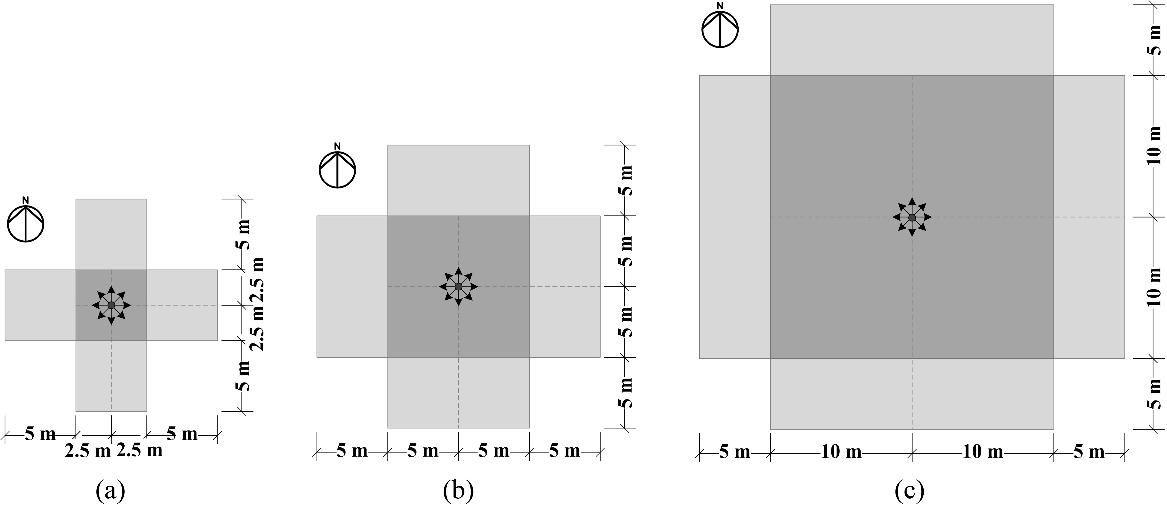
Fig. 1. Plan view of the courtyard scenes with the square size s of (a) 5 m, (b) 10 m, and (c) 20 m.

The second scene involves a street canyon surrounded with two parallel building blocks of equal height. In this case, the street width w is either 5 or 10 m, typically representing the situation in urban residential areas [23,24]. The building blocks have an equal height h of 3, 6, or 9 m, and are placed either in the north and south of the street (i.e. the street has east-west direction) or in the east and west of the street (i.e. the street has north-south direction), as shown in Fig. 2.

Figure 2

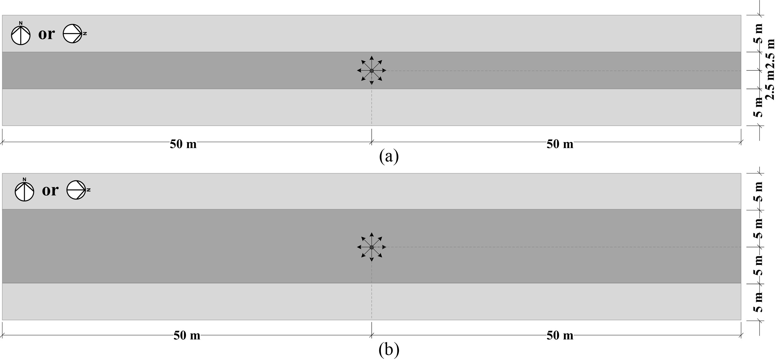
Plan view of the street canyon scenes with the street width w of (a) 5 m and (b) 10 m. In each scene, the building blocks are positioned either in the north and south (N-S) or in the east and west (E-W) of the street.

Fig. 2. Plan view of the street canyon scenes with the street width w of (a) 5 m and (b) 10 m. In each scene, the building blocks are positioned either in the north and south (N-S) or in the east and west (E-W) of the street.

As reference, a baseline scene comprising only a ground without any building is also created. In all scenes, the receiving point is at 1.5 m high from the ground (or street level), representing typical eye height for a standing adult, in the centre of the courtyard or of the street (Fig. 3). The illuminance sensors at that point are placed on the horizontal and vertical planes. The latter are set to face north, northeast, east, and so forth until northwest, so that there are nine receiving planes (1 horizontal, 8 vertical) in each scenario. The building blocks and the ground are modelled to have a spectrally neutral reflectance of respectively 0.5 and 0.2. Based on the literature [25], there is a large variation of reflectance values for actual building exterior materials, ranging from 0.1 to 0.9, thus 0.5 represents the middle value. The value of 0.5 can be attributed to beige-coloured concrete or ceramics [25].

Figure 3

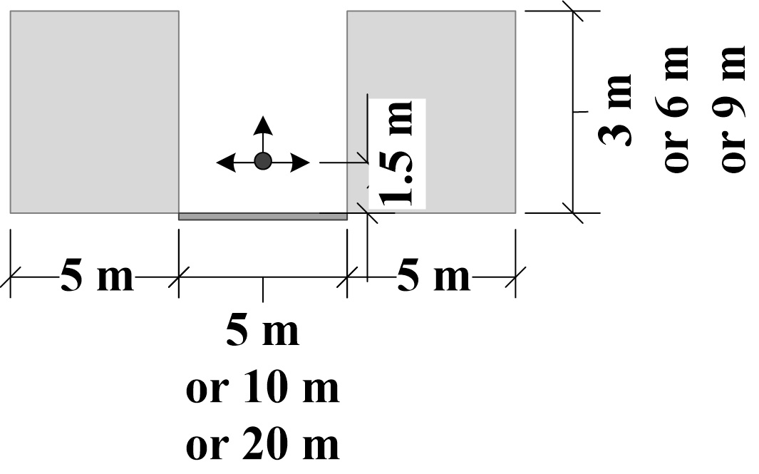
Section view of the courtyard and street canyon scenes. In both scenes, the building height is varied within 3, 6, and 9 m; whereas the receiving point is 1.5 m high above the ground.

Fig. 3. Section view of the courtyard and street canyon scenes. In both scenes, the building height is varied within 3, 6, and 9 m; whereas the receiving point is 1.5 m high above the ground.

Based on the aforementioned description of the modelled scenarios, there are therefore 22 scenarios modelled in this study, i.e. 1 baseline scene, 9 courtyard scenes (3 s combinations × 3 h), and 12 street canyon scenes (2 w × 3 h × 3 building blocks orientations). Table 1 summarises all of these scenarios.

Table 1

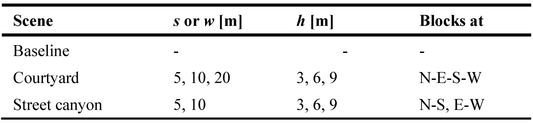
Table 1. Summary of all modelled scenarios.

The location is set in the city of Bandung, Indonesia (6.93°S, 107.61°E), located in the Af (tropical rainforest) climate region according to the Köppen–Geiger climate classification. The city is located approximately 750 m above sea level, and thus is relatively cooler than most other Indonesian large cities, but can be of high risk in terms of UV radiation due to the tropical location and its high altitude. The weather data file in EPW format was provided by the Institute of Research and Development for Dwellings, the Ministry of Public Work and Housing of the Republic of Indonesia, based on measurements during the years 1997~2004.

The measurements were conducted continuously using a dedicated weather monitoring system installed in an open field, at the site of the Institute, located in the eastern part of Bandung Greater Metropolitan area. Relevant weather parameters were collected, including dry bulb and dew point temperatures, relative humidity, barometric pressure, solar irradiance, wind speed and direction, and precipitation depth. The associated data file is indeed a typical meteorological year (TMY), in which data for different months are extracted from different years within the years 1997~2004. In details, the data are extracted from January and February 1999, March 1997, April 1999, May 1997, June 2004, July 2001, August 2004, September 2003, October 2004, November 1999, and December 2003.

The building geometry and material properties are created and defined in Radiance as a *.rif file and are imported to Daysim to perform the annual daylighting analysis, using a time step of 5 min. The ambient simulation parameters [10] are summarised in Table 2, which corresponds to accurate~maximum setting for Radiance/Daysim calculations, to ensure high accuracy of the results. To give an idea on how the selected surrounding building typologies actually look in the real context, Fig. 4 displays several real images of courtyards and street canyons in the city of Bandung.

Table 2

Table 2. Daysim simulation parameters [10].

Figure 4

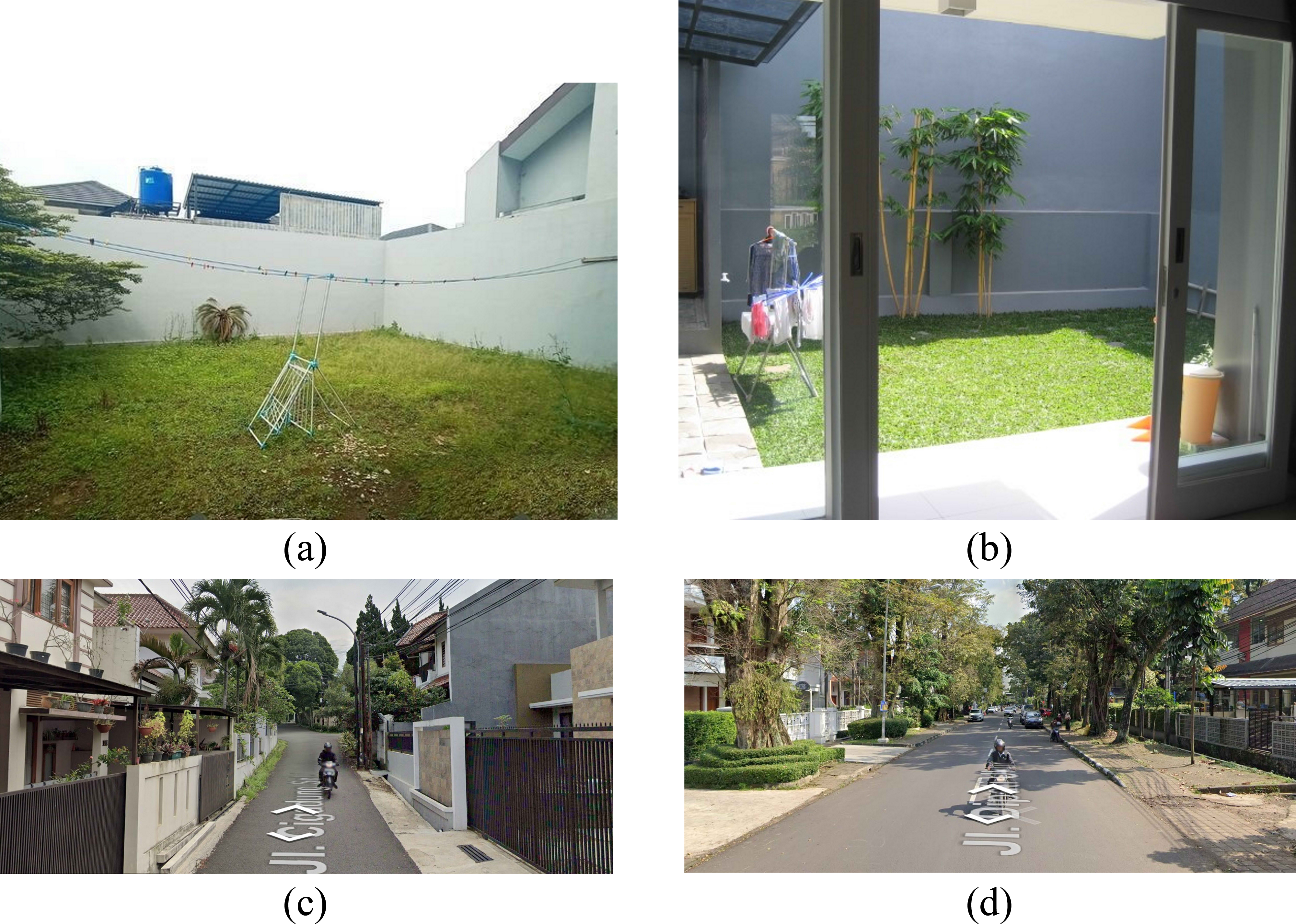
Real images examples of (a) courtyard with h ≈ 3 m (source: https://www.jualo.com), (b) courtyard with h ≈ 6 m (source: https://rumahdijual.com), (c) street canyon with w ≈ 5 m (source: https://www.instantstreetview.com, © 2020 Google), (d) street canyon with w ≈ 10 m (source: https://www.instantstreetview.com, © 2020 Google), in the urban area of the city of Bandung.

Fig. 4. Real images examples of (a) courtyard with h ≈ 3 m (source: https://www.jualo.com), (b) courtyard with h ≈ 6 m (source: https://rumahdijual.com), (c) street canyon with w ≈ 5 m (source: https://www.instantstreetview.com, © 2020 Google), (d) street canyon with w ≈ 10 m (source: https://www.instantstreetview.com, © 2020 Google), in the urban area of the city of Bandung.

The performed simulations yield the annual profile consisting of global illuminance (E_v,g, in lx) data for all receiving planes, reported from 1 January to 31 Dec at every 5 min. In this case, since one is interested to observe only the morning-time profile, only the data between 08.00 and 12.00 hrs are analysed. To simplify the presentation, the median of annual E_v,g for each scenario is reported in Section 3, as a function of time stamp (08.00~12.00 hrs), separated in terms of the receiving plane (i.e. horizontal and the eight vertical planes).

To appreciate the seasonal variation, the daily E_v,g profile for each scenario is reported for the dates of 21 March, 21 June, and 22 December, to represent the equinox and the two solstices. Again, the profile is shown for the period of 08.00~12.00 hrs, also separated in terms of the receiving plane.

2.2. Conversion to global irradiance

Since the simulation results in Daysim only comprises E_v,g data for the selected time step, conversion to global irradiance (E_e,g, in W/m²) is required as an intermediate step to predict the risk of sunlight exposure. To do so, the global luminous efficacy K_g is to be determined by dividing the obtained hourly E_v_,g data on horizontal plane from the simulation of the baseline scene (no surrounding buildings) with the corresponding hourly E_e_,g (also on horizontal plane) from the EPW data file, which has been provided in 1-hour time step. The instantaneous K_g is assumed constant for horizontal and vertical planes in scenes with surrounding buildings, at the given hour mark.

However, the Daysim simulations are performed in 5-min time step, so that the daily profile would have a high resolution. Therefore, interpolation is necessary to determine the appropriate K_g for any time stamp located between two full hour marks. In other words, the K_g at time t = H+m, where H denotes the hour mark and m denotes the minutes past the hour, can be determined based on Eq. (1) as follows:

\[ \left.\ K_g\right|_{t=H+m}=\left.\ K_g\right|_{t=H}+\frac{m}{60}\left(\left.\ K_g\right|_{t=H+1}-\left.\ K_g\right|_{t=H}\right) \]

Based on the definition of luminous efficacy, the E_e,g value on any receiving plane at time t = H+m is therefore:

\[ \left.\ E_{e,g}\right|_{t=H+m}=\frac{\left.\ E_{v,g}\right|_{t=H+m}-B}{A} \]

Alternatively, the conversion between E_v,g and E_e,g can also be realised by pairing the hourly data for the entire year in a scatter plot. The resulting trend is likely to be linear, as suggested in past daylighting studies in the tropics [26,27]. In that case, E_v,g = AE_e,g + B, where A and B are coefficients to be determined from the empirical relation. Thus, assuming such linear model holds for any given time of the year, one can estimate:

\[ \left.\ E_{e,g}\right|_{t=H+m}=\frac{\left.\ E_{v,g}\right|_{t=H+m}-B}{A} \]

It can be shown later that the estimated E_e_,g values obtained from Eqs. (2) and (3), for the selected climate, are relatively close to each other.

2.3. Conversion to UV index

The risk of sunlight exposure to human can be indicated with the UV index (UVI), which is a simplified scale indicating the relative strength of solar UV radiation. The UVI is generally used as a precaution to take necessary protection when one is to be exposed to outdoor sunlight. Technically, UVI is as a weighted representation of the total incident flux of UV radiation in the biologically active range of 280~400 nm [28-31]; whereas the range below 280~290 nm may be excluded due to its negligible contribution [32]. The relevant weighting is the so-called erythema action spectrum (EAS(λ)) [30,33,34], which reads:

\[ \mathrm{EAS}(\lambda)=\left\{\begin{matrix}1,\mathrm{\ \ \ \ \ \ \ \ \ \ \ \ \ \ \ \ \ \ }250\mathrm{\ nm}\le\lambda\le298\mathrm{\ nm}\\10^{0.094(298-\lambda)},\mathrm{\ \ }\ 298\mathrm{\ nm}\ <\lambda\le328\mathrm{\ nm}\ \\10^{0.015(140-\lambda)},\mathrm{\ \ }\ 328\mathrm{\ nm}\ <\lambda\le400\mathrm{\ nm}\ \\\end{matrix}\right. \]

The UVI is the product of the EAS(λ) based on Eq. (4) and the incident irradiance (E_e(λ)) on the receiving surface, integrated over the spectral range of 280~400 nm that represents UV-A and UV-B, and is scaled by a factor of 1/(25 mW/m²) [29,35,36], so that:

\[ \mathrm{UVI}=\frac{1}{25\mathrm{\ mW/}\mathrm{m}^2}\int_{280\mathrm{\ nm}}^{400\mathrm{\ nm}}{E_e(\lambda)\cdot}\mathrm{\mathrm{\ }EAS(\lambda)\cdot d\lambda.} \]

The UVI value from Eq. (5) typically ranges between 0 and 11, although values greater than 11 is not uncommon particularly in the tropical region, where the solar elevation angle is high at around noon, and also in places with high altitude, where the atmospheric optical path is relatively shortened compared to that with low altitude [29]. UVI values between 0 and 2 are considered ‘low’ risk, between 3 and 5 are ‘moderate’, between 6 and 7 are ‘high’, between 8 and 10 are ‘very high’, and those exceeding 11 are ‘extreme’ [29,35,36].

In the standard format of EPW file, UVI is typically not included. However, Eq. (5) suggests that UVI is proportional to incident solar irradiance. The complete spectrum of E_e(λ) is also never reported in the EPW file, but the temporal data of horizontal E_e,g integrated over the whole UV, visible, and near infrared wavelengths are available. To determine the typical range of UVI at the particular location, an empirical model is drawn (Fig. 5) based on the continuous measurement of the maximum daily UVI and maximum daily horizontal E_e,g within the period of May 2019~April 2020 in the rooftop of Labtek IXB Building in ITB Campus in Bandung (data are available in Ref. [37]). The UV measuring instrument is Davis Instruments with Vantage Pro2^TM sensor, having the spectral response from 290 to 390 nm, measures at 1 scale resolution. The pyranometer is Davis Instruments 6450 with Vantage Pro2^TM sensor, measures at 1 W/m² resolution, range 0~1800 W/m², with the spectral response (10% points) is from 400 to 1100 nm. The sensor accuracy ±5% of full scale, with drift up to ±2% per year.

Figure 5

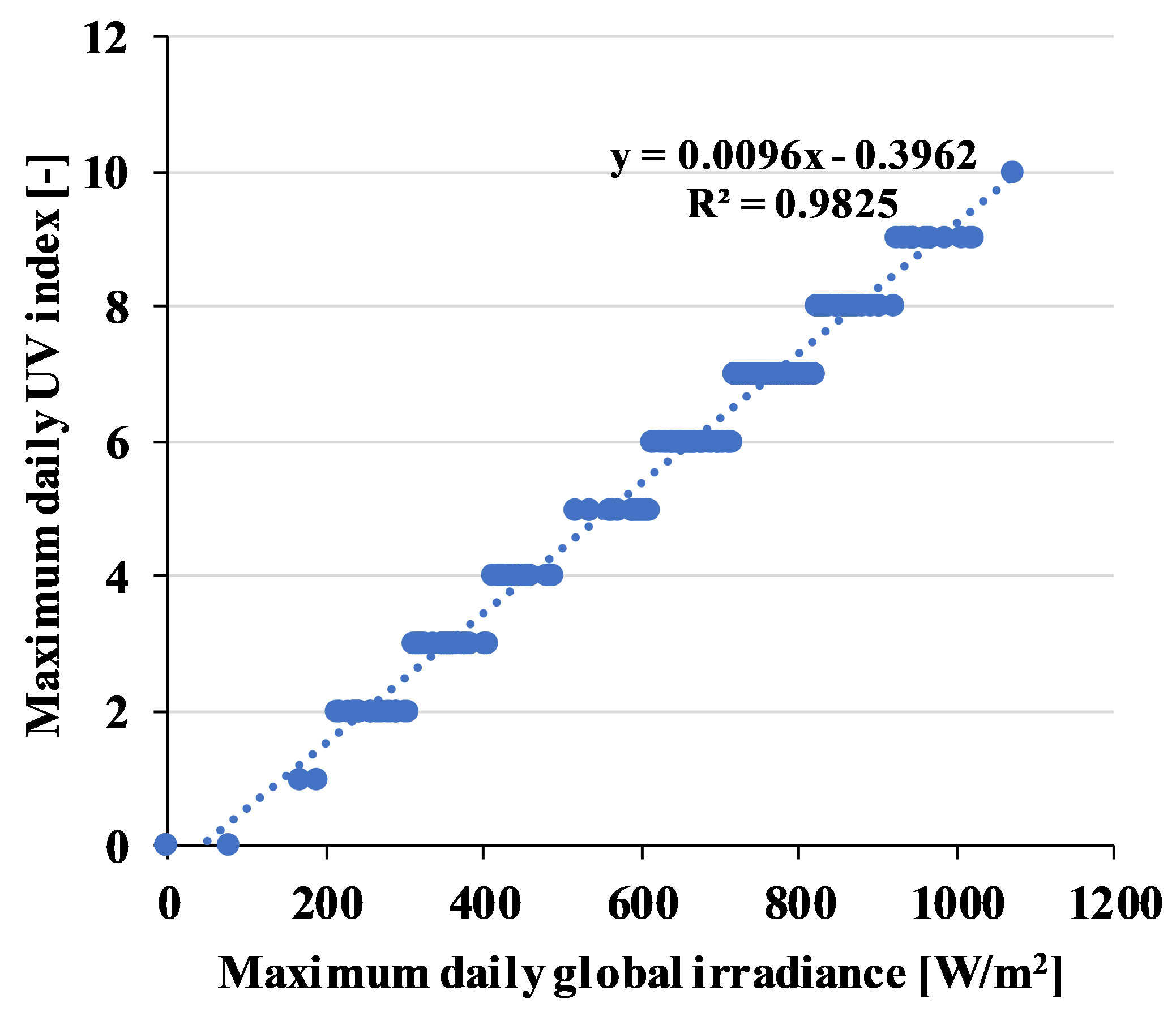
Empirical relation between maximum daily UV index and maximum daily global horizontal irradiance measured continuously within the period of May 2019~April 2020 in Bandung.

Fig. 5. Empirical relation between maximum daily UV index and maximum daily global horizontal irradiance measured continuously within the period of May 2019~April 2020 in Bandung.

After performing linear regression (R² = 0.9825) to the obtained data, the following local model in Eq. (6) is obtained:

\[ UVI = 0.0096\ E_{e,g} – 0.3962 \]

Figure 6(a) displays the hourly E_e_,g on horizontal plane as provided in the employed EPW climate data of Bandung, from 1 January to 31 December. Meanwhile, Fig. 5(b) displays the corresponding, estimated UVI based on Eq. (3), assuming it holds for the entire EPW climate data, rounded to the nearest integer. Figure 6(b) suggests that none of the estimated UVI exceeds 11; i.e. there is no situation with extreme risk in the entire year, which is also confirmed by the recent actual measurement in Fig. 5. Since climate data are typically extracted from measurement in an open field, once the data are applied to estimate the daylighting profile at points with surrounding buildings, the resulting UVI are not expected to be higher than those in Fig. 6(b).

Figure 6

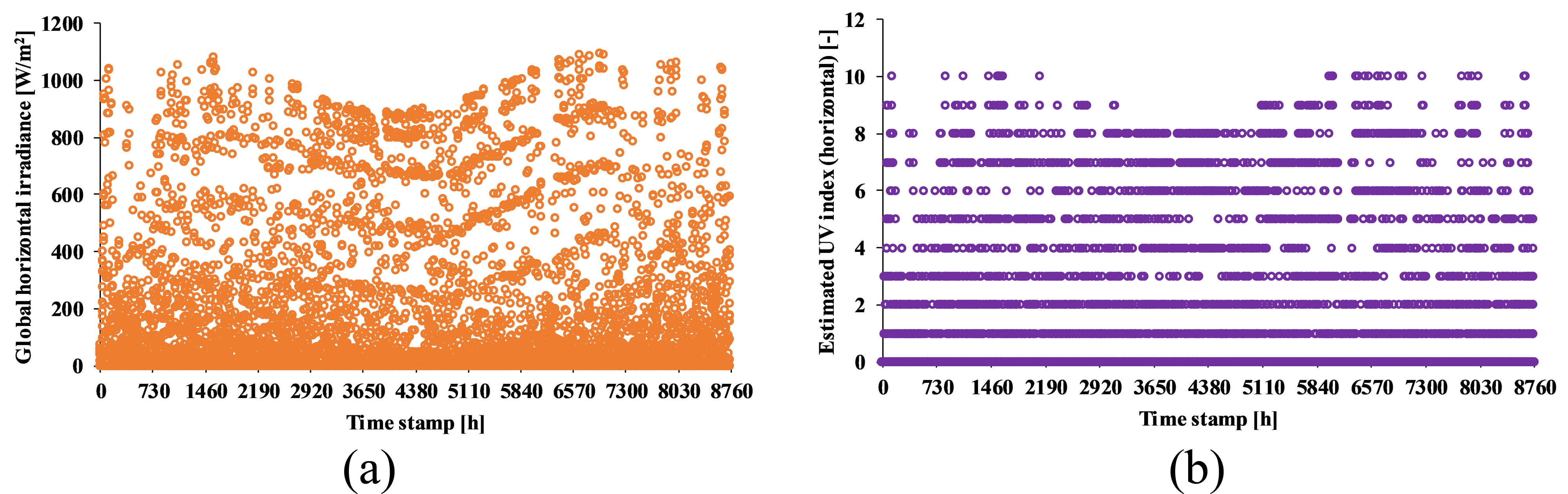
Fig. 6. (a) Hourly global horizontal irradiance as provided in the employed EPW climate data of Bandung, and (b) the corresponding, estimated UV index.

Having known the relation between UVI and E_e_,g, Eqs. (2) and (3) can be recalled to estimate UVI at time t = H+m, by substituting E_e_,g in Eq. (6) in two different ways, i.e.:

\[ \left.\ \mathrm{UVI}\right|_{t=H+m}\approx0.0096\frac{\left.\ E_{v,g}\right|_{t=H+m}}{\left.\ K_g\right|_{t=H+m}}-0.3962 \]

and:

\[ \left.\ \mathrm{UVI}\right|_{t=H+m}\approx0.0096\frac{\left.\ E_{v,g}\right|_{t=H+m}-B}{A}-0.3962 \]

To indicate the risk of UV radiation in the representative days of 21 March, 21 June, and 22 December within 08.00~12.00 hrs, the peak times at which the maximum E_v_,g is achieved are reported, for horizontal and the eight vertical planes, in the baseline, courtyard, and street canyon scenes. The corresponding UVI values for each plane are then estimated using both Eqs. (7) and (8), for all scenes.

2.4. Sensitivity analysis

2.4. Sensitivity analysis

To systematically determine the influence of the input parameters of the surrounding buildings on the estimated UVI, sensitivity analysis is conducted by performing multiple linear regressions, considering either only the three selected days (21 March, 21 June, and 22 December), or all days in the entire year.

For the courtyard scene, the involved input parameters are: size s and height h of the courtyard, and the order of the particular day in the year (d, for instance 21 March has d = 81). For the street canyon scene, the involved input parameters are: street width w, building blocks’ height h, street orientation α (0° for street with east-west building blocks, and 90° for street with north-south building blocks), and the order of the particular day in the year (d).

The output parameters are the daily maximum estimated UVI on the horizontal plane; and the daily maximum estimated UVI among the entire vertical planes. Eq. (8) is employed to estimate the UVI directly from the simulated E_v,g data.

Before performing the regression, all input (x_i) and output (y_i) parameters are normalised with respect to the mean (μ_x and μ_y) and standard deviation (σ_x and σ_y) values, based on Eq. (9) as follows:

\[ x\prime_i=\frac{x_i-\mu_x}{\sigma_x}\mathrm{\ \ ;\ \ \ }y\prime_i=\frac{y_i-\mu_y}{\sigma_y} \]

The regression analysis for the courtyard scene is performed according to the model in Eq. (10):

\[ \mathrm{UVI}\prime=\beta_1\prime\ s\prime+\beta_2\prime\ h\prime+\beta_3\prime\ d\prime+\varepsilon \]

where UVI’ is to be substituted with the normalised, estimated maximum horizontal and vertical UVI; β’ is the standardised regression coefficient (SRC), and ε is the residual error.

The regression analysis for the street canyon scene is performed according to the model in Eq. (11):

\[ \mathrm{UVI}\prime=\beta_1\prime\ w\prime+\beta_2\prime\ h\prime+\beta_3\prime\alpha\prime+\beta_4\prime\ d\prime+\varepsilon \]

where y’ is also to be substituted with the normalised, estimated maximum horizontal and vertical UVI. The influence of each input parameter on the output is characterised with its SRC, where SRC = 1 represents a highly positive influence, SRC = –1 represents a highly negative influence, and SRC = 0 represents no influence at all.

3. Results

3.1. Global illuminance profiles

3.1.1. Baseline scene

Figure 7 displays the estimated median of annual global illuminance E_v,g in the baseline scene, whereas Fig. 8 displays the daily profile of E_v,g within 08.00~12.00 hrs on 21 March, 21 June, and 22 December in the same scene, based on the obtained results from Daysim simulation. The profiles are shown separately for horizontal (Hor) and the eight vertical planes (facing north (N), northeast (NE), and so forth).

Figure 7

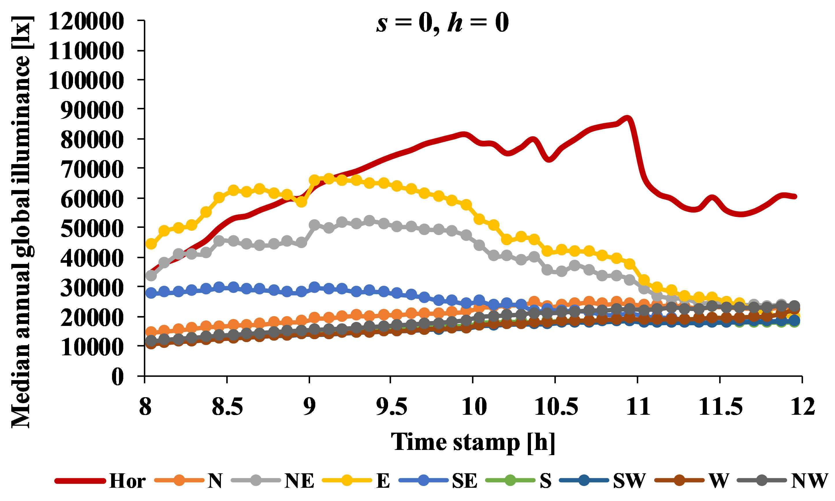
Fig. 7. Estimated median of annual global illuminance within 08.00~12.00 hrs in the baseline scene.

Figure 8

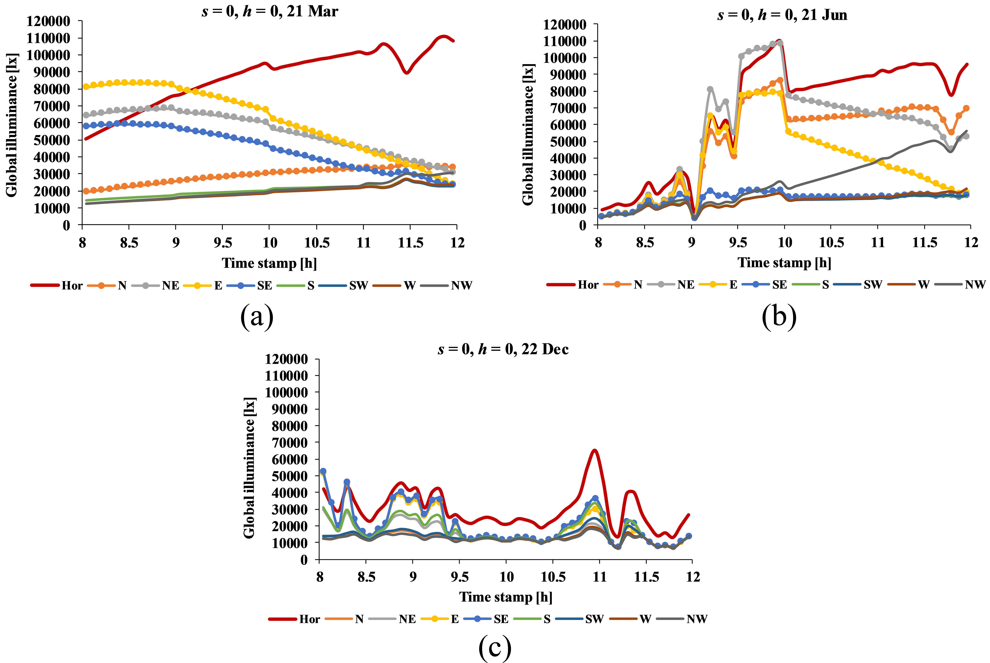
Fig. 8. Estimated global illuminance within 08.00~12.00 hrs in the baseline scene on (a) 21 March, (b) 21 June, and (c) 22 December.

Figure 7 suggests that between 09.00 and 12.00 hrs, the E_v,g values on the horizontal plane (E_v,g_,hor) are expected to be greater than E_v,g on any of the vertical planes. However, between 08.00 and 12.00 hrs, the vertical E_v,g facing east (E_v,g_,E) are expected to be greater due to the low solar elevation angle. The expected peak time for E_v,g_,hor is at around 11.00 hrs, whereas that for E_v,g_,E is at around 09.00 hrs. The peak value for the latter (66000 lx) is approximately 77% as large as the former (86500 lx). The northeast and southeast orientations also have distinct profiles, though lower than the E_v,g_,E profile. The remaining orientations are relatively similar to each other and receive relatively small E_v,g values, ranging from 10000 to 23000 lx throughout the morning.

The daily E_v,g profiles on the three selected days reveal some relevant information. Among those days, the profile on 21 March (Fig. 8(a)) is virtually the closest to the median annual profile, in terms of peak times and values. The only difference is perhaps that the north orientation also appears to have a distinct profile so that E_v,g_,N < E_v,g_,SE < E_v,g_,NE < E_v,g_,E within 08.00~10.30 hrs. Notice that 21 March represents the equinox, in which the sun is at its closest position to the equator. The profile on that day also resembles a typical day with intermediate sky, which is dominant (around 78%) in Indonesian climate [38,39]. For a given data set, the median can be thought as the middle value, which may better represent the ‘typical’ value, because it would not change dramatically by a small proportion of extremely small or large data values, as would happen to the mean (or average) value. In this case, because the resulting global illuminance data vary greatly between days in a year, the mean value for each time stamp would be sensitive to the occurrence of extreme values, and thus may not well describe the typical daily profile. This choice is further justified by the daily profile of E_v,g on 21 March in the baseline scene (Fig. 8(a)) that closely resemble the profile of annual E_v,g in the same scene (Fig. 7).

The profile on 21 June (Fig. 8(b)) represents situation with a rather clear sky in the morning, with the peak time lies between 09.30 and 10.00 hrs. Within that frame, the E_v,g_,NE almost has the same trends and values (around 110000 lx) with E_v,g_,hor, if not greater. The E_v,g_,E and E_v,g_,N values become the second and third highest within that time frame, but the former quickly diminish towards noon, whereas the latter relatively maintain at 70000~80000 lx.

Finally, the profile on 22 December (Fig. 8(c)) represents a typical overcast sky scenario in the tropics, which is characterised with high amount of rainfalls and high percentage of cloud cover. The peak E_v,g is achieved at around 11.00 hrs, receiving only approximately 60000 lx on the horizontal plane, about half of the maximum amount in 21 June. Variations between the vertical orientations are not distinct in that time of the year, with the southeast orientation (E_v,g_,SE) being the closest to the E_v,g_,hor.

3.1.2. Courtyard and street canyon scenes

The estimated median of annual E_v,g in the nine scenarios for the courtyard scenes, based on Daysim simulation results, are displayed in Fig. 9. Among these scenarios, it is observed that those with h = 3 m have approximately similar annual profile, and so the reduction due to shading is not clearly visible. The shading effect is nonetheless significant in scenes with s = 5 m, which is sensitive to height variation. For h = 3 m, the maximum E_v,g at

Figure 9

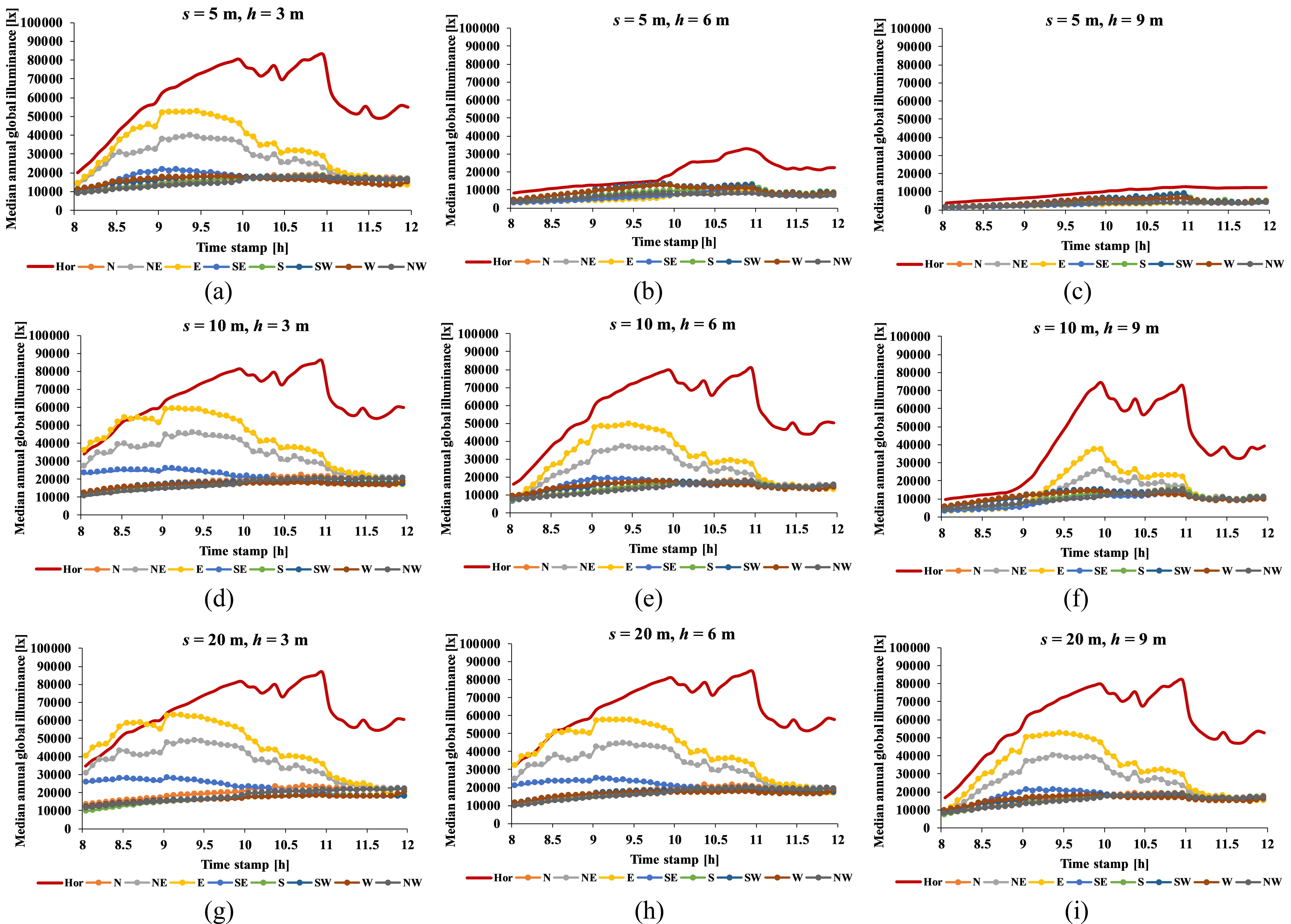
Estimated median of annual global illuminance within 08.00~12.00 hrs in the courtyard scenes with: (a) s = 5 m, h = 3 m, (b) s = 5 m, h = 6 m, (c) s = 5 m, h = 9 m, (d) s = 10 m, h = 3 m, (e) s = 10 m, h = 6 m, (f) s = 10 m, h = 9 m, (g) s = 20 m, h = 3 m, (h) s = 20 m, h = 6 m, (i) s = 20 m, h = 9 m.

Fig. 9. Estimated median of annual global illuminance within 08.00~12.00 hrs in the courtyard scenes with: (a) s = 5 m, h = 3 m, (b) s = 5 m, h = 6 m, (c) s = 5 m, h = 9 m, (d) s = 10 m, h = 3 m, (e) s = 10 m, h = 6 m, (f) s = 10 m, h = 9 m, (g) s = 20 m, h = 3 m, (h) s = 20 m, h = 6 m, (i) s = 20 m, h = 9 m.

around 11.00 hrs is 80000 lx, but the value is reduced to 35000 lx for h = 6 m, and is further reduced to 12000 lx for h = 9 m. In the latter two scenarios, the vertical planes orientation is not important since the vertical E_v,g values at any given time are highly similar with each other (Figs. 9(b) and (c)).

In the larger courtyard scenes (s = 10 or 20 m), the increasing height gives less contribution in reducing the E_v,g, thus less shading effect compared to the 5-m size courtyard. However, between 08.00 and 09.00 hrs, E_v,g reduction can be observed, particularly on the horizontal, east-facing, and northeast-facing vertical planes. In all scenarios, except in s = 5 m with h ≥ 6 m, the maximum E_v,g on the vertical planes is received when facing east, followed by northeast. The peak time frame is found within 09.00~10.00 hrs, with the values dramatically reduced afterward.

Meanwhile, Fig. 10 displays the estimated median of annual E_v,g in the street canyon scenes, all within 08.00~12.00 hrs, based on Daysim simulation results. The 5-m wide street (i.e. the narrow one) is found to be more sensitive to height variation, compared to the 10-m wide (i.e. the wide one). For w = 5 m and h = 3 m, the maximum E_v,g_,hor is 80000 lx at around 11.00 hrs, for both orientations of the building blocks. The maximum vertical E_v,g values are around 55000 lx facing east in the east-west (E-W) blocks scene and 60000 lx facing east in the north-south (N-S) one, at around 09.00 hrs, due to direct sunlight from the east.

Figure 10

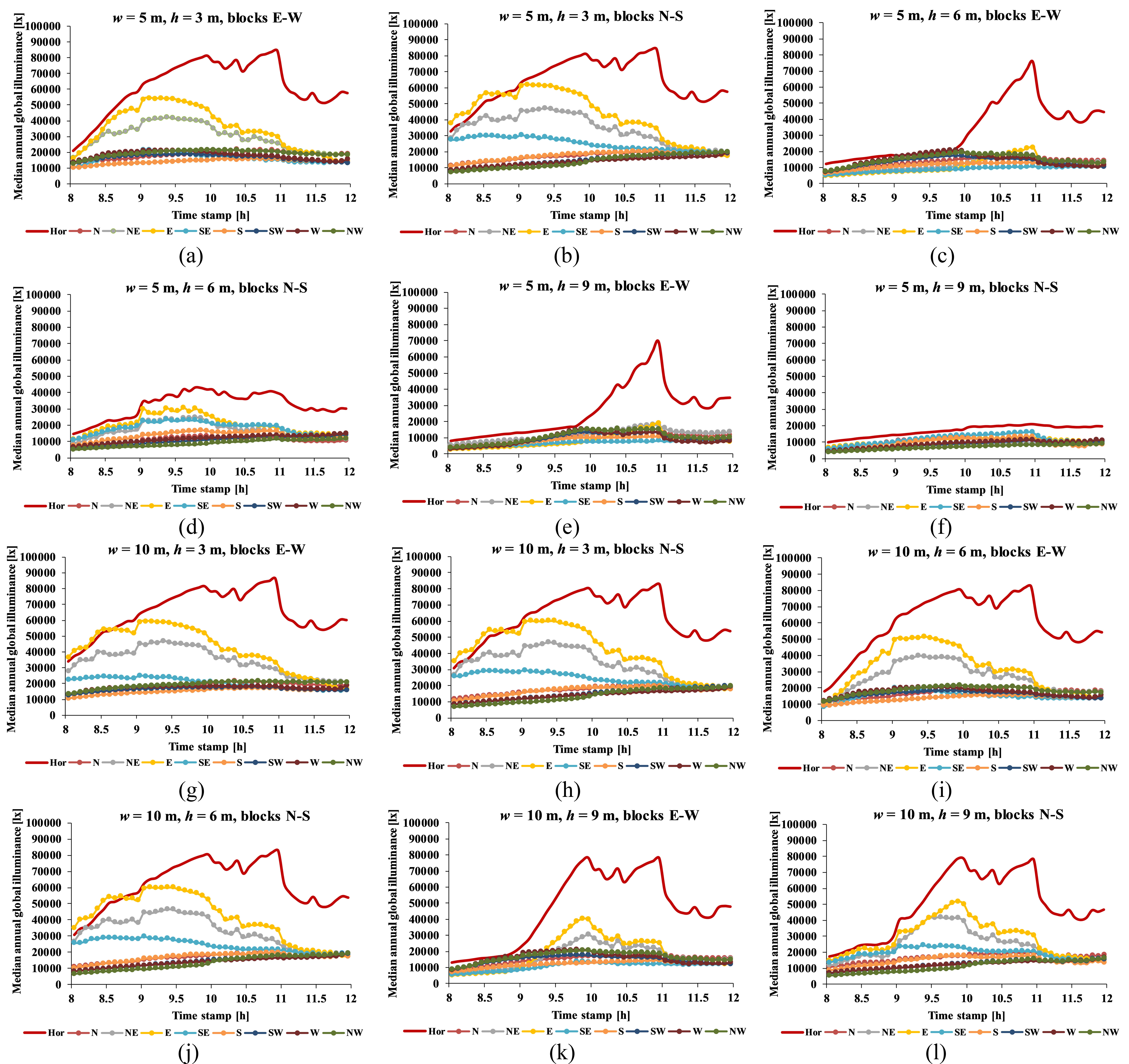
Estimated median of annual global illuminance within 08.00~12.00 hrs in the street canyon scenes with: (a) w = 5 m, h = 3 m, blocks in east and west (E-W), (b) w = 5 m, h = 3 m, blocks in north and south (N-S), (c) w = 5 m, h = 6 m, E-W, (d) w = 5 m, h = 6 m, N-S, (e) w = 5 m, h = 9 m, E-W, (f) w = 5 m, h = 9 m, N-S, (g) w = 10 m, h = 3 m, E-W, (h) w = 10 m, h = 3 m, N-S (i) w = 10 m, h = 6 m, E-W, (j) w = 10 m, h = 6 m, N-S, (k) w = 10 m, h = 9 m, E-W, (l) w = 10 m, h = 9 m, N-S.

Fig. 10. Estimated median of annual global illuminance within 08.00~12.00 hrs in the street canyon scenes with: (a) w = 5 m, h = 3 m, blocks in east and west (E-W), (b) w = 5 m, h = 3 m, blocks in north and south (N-S), (c) w = 5 m, h = 6 m, E-W, (d) w = 5 m, h = 6 m, N-S, (e) w = 5 m, h = 9 m, E-W, (f) w = 5 m, h = 9 m, N-S, (g) w = 10 m, h = 3 m, E-W, (h) w = 10 m, h = 3 m, N-S (i) w = 10 m, h = 6 m, E-W, (j) w = 10 m, h = 6 m, N-S, (k) w = 10 m, h = 9 m, E-W, (l) w = 10 m, h = 9 m, N-S.

For w = 5 m and h = 6 m, the maximum E_v,g_,E in the N-S scene is reduced by half compared to w = 5 m and h = 3 m, and is further reduced by half when h = 9 m. In other words, a narrow street with high surrounding blocks will ensure the least amount of vertical E_v,g, and thus also E_e,g and estimated UVI, even on the east-facing plane. Moreover, when w = 5 m and h = 9 m, the impact of orientation on the vertical E_v,g is little, in which the E-W scene receives larger maximum E_v,g_,hor (70000 lx) compared to the N-S scene (20000 lx), at around 11.00 hrs.

In the scenarios with wider street width w = 10 m, the impact of building height is subtle, i.e. there is less shading effect, at least for the E_v,g_,hor, except in the early morning between 08.00 and 09.00 hrs. The first four scenarios with w = 10 m (Figs. 10(g) until (j)) result in relatively similar median profiles. For h = 9 m, the reduction in vertical E_v,g is more visible, with the peak at around 10.00 hrs. In all 10-m wide street scenarios, the maximum vertical E_v,g are achieved when facing east, followed by northeast. In general, a wider street would receive larger vertical E_v,g and estimated UVI, compared to the narrower one in a urban residential area.

3.2. UV index estimation

To estimate the UVI, the relation between E_v,g in the baseline scene and E_e,g in the EPW data file is observed, as described in Section 2.2. Figure 11(a) shows the resulting scatter plot, whereas Fig. 10(b) displays the hourly profile of the resulting K_g from 1 January to 31 December.

As expected, Fig. 11(a) suggests a linear relationship (R² = 0.993) between E_v_,g and E_e_,g, which reads in Eq. (12) as follows:

\[ E_{v,g}\ \ =\ 107.97\ E_{e,g}\ – 269.64, \]

so that A and B coefficients in Eq. (3) are now known. Fig. 11(b) also suggests that the hourly K_g values mostly vary within between 98 lm/W (the first percentile) and 137 lm/W (the 99^th percentile). The median value is 114 lm/W, while the lower and upper quartiles are respectively 109 and 125 lm/W.

Figure 11

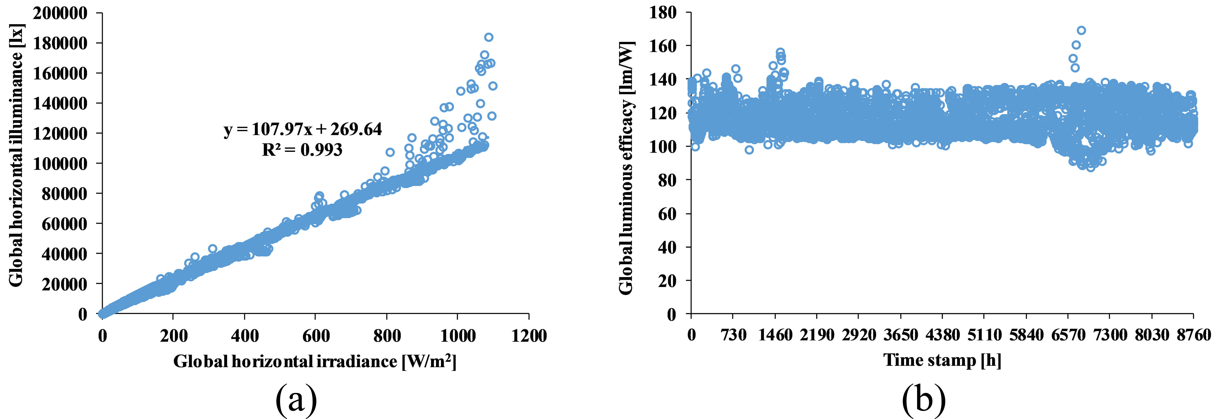
Fig. 11. (a) Relation between global horizontal illuminance and irradiance, and (b) hourly luminous efficacy as obtained in the baseline scene.

Based on the obtained daily profiles of E_v_,g from simulations in the three selected days, the peak times at which the maximum E_v_,g are found can be identified. Using either Eq. (2) or (3), the UVI for those peak times can therefore be estimated. If Eq. (3) is assumed, the instantaneous UVI in the particular location can simply be estimated from the corresponding E_v_,g as in Eq. (13):

\[ \left.\ \mathrm{UVI}\right|_{t=H+m}\approx8.89\times10^{-5}\left.\ E_{v,g}\right|_{t=H+m}-0.42 \]

In cases where both equations yield different UVI values, both of them are reported. It is noticed however that in such cases, the two estimated values of UVI would differ only by one scale, and so is the estimated uncertainty, provided the same EPW data.

Tables 3, 4, and 5 summarise the estimated UVI, rounded to the nearest integer, respectively for the baseline, courtyard, and street canyon scenes. Note that for the vertical planes, only the orientation giving the maximum E_v_,g, and thus also the maximum UVI, is reported. Given the linear relation between UVI and E_v_,g, the annual profile of the UVI values in the baseline scene assumes the same shape with that of the E_v_,g in the same scene. For efficiency, the annual UVI profile in the baseline scene is thus not presented. Nonetheless, the peak values of median E_v_,g and the corresponding UVI values in the baseline scene are also reported in Table 3.

Table 3

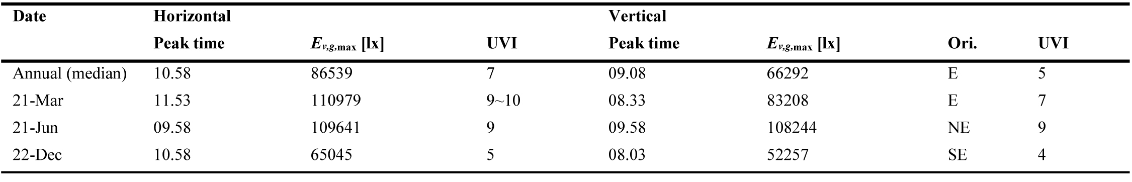
Table 3. Estimated peak time (hh.mm) of global horizontal and vertical illuminance and the corresponding UV index for the baseline scene.

Table 4

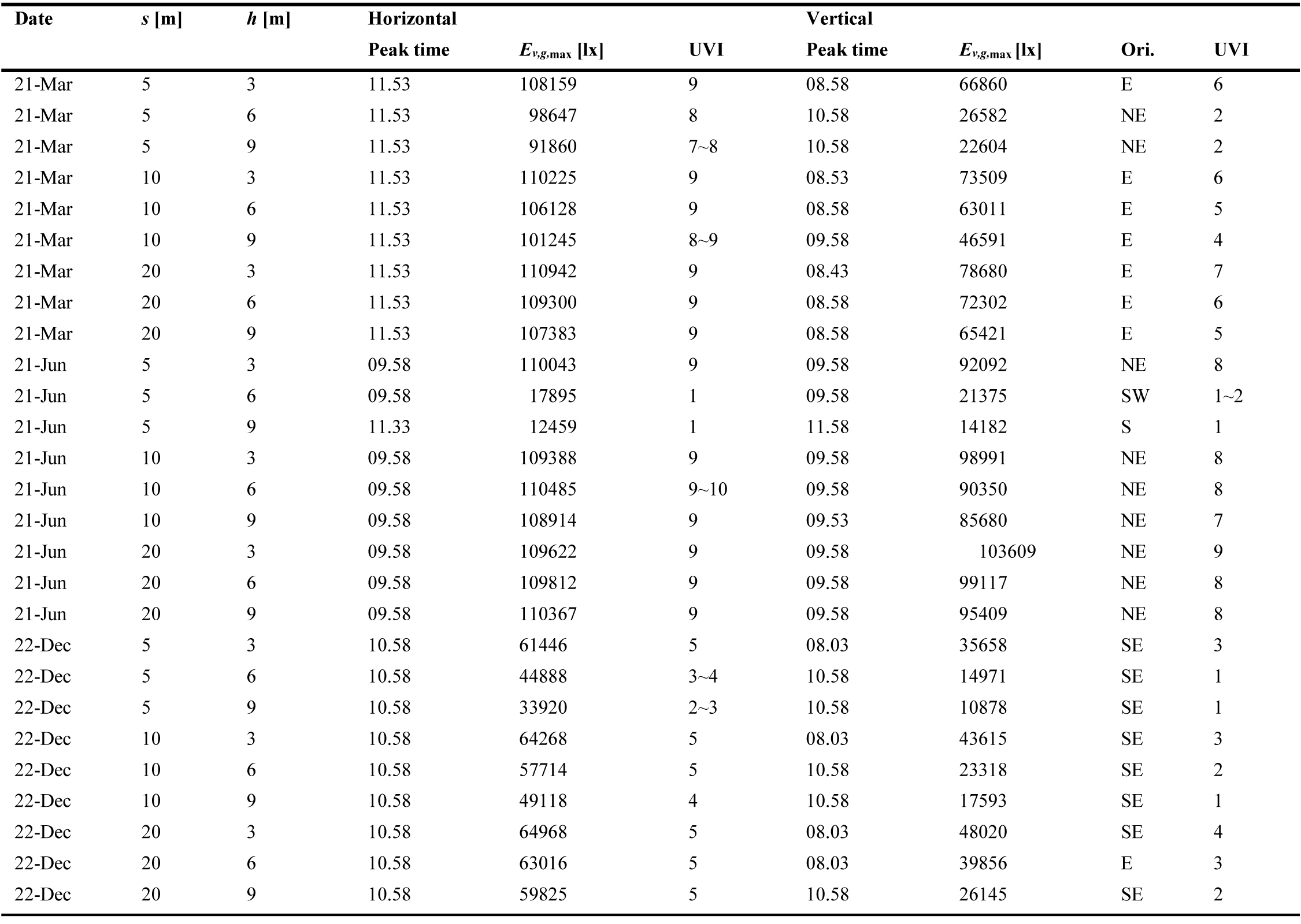
Table 4. Estimated peak time (hh.mm) of global horizontal and vertical illuminance and the corresponding UV index for the courtyard scenes.

Table 5

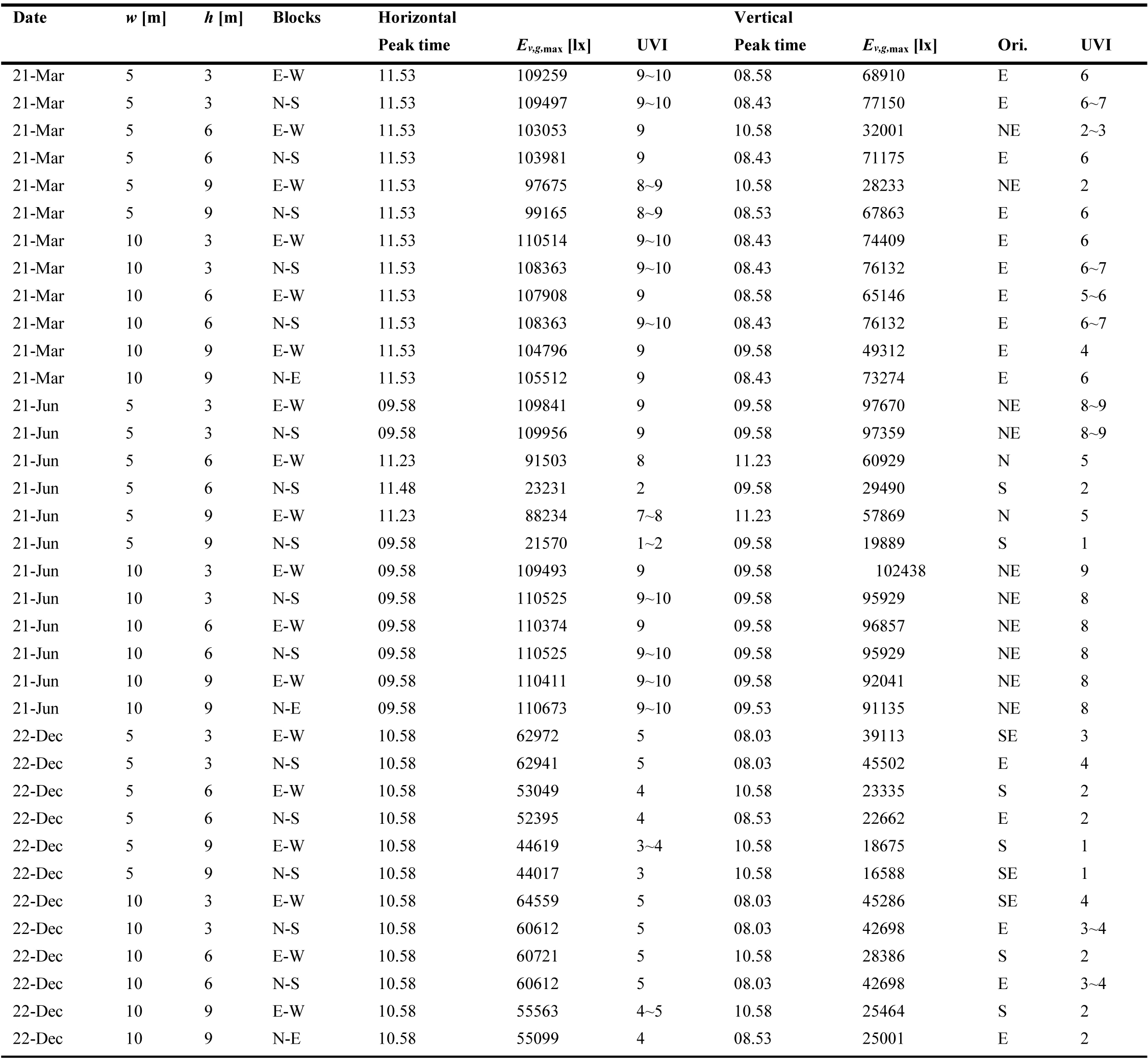
Table 5. Estimated peak time (hh.mm) of global horizontal and vertical illuminance and the corresponding UV index for the street canyon scenes.

Based on Table 4, the courtyard scenario that yields the maximum UVI on the selected three days is s = 10 m and h = 3 m. In this scenario, the estimated UVI on the horizontal plane on 21 March, 21 June, and 22 December are respectively 9, 9, and 5. Meanwhile, based on Table 5, the street canyon scenario yielding the maximum UVI is w = 10 m, h = 3 m, with building blocks in the east and west (i.e. street direction north-south); so that the estimated horizontal UVI on 21 March, 21 June, and 22 December are respectively 9~10, 9, and 5.

To visualise the daily profiles of the courtyard and street canyon scenarios having the maximum UVI, Figs. 12 and 13 display the estimated UVI values using Eq. (13). The profiles are given within 08.00~12.00 hrs for both scenarios on the three selected days.

Figure 12

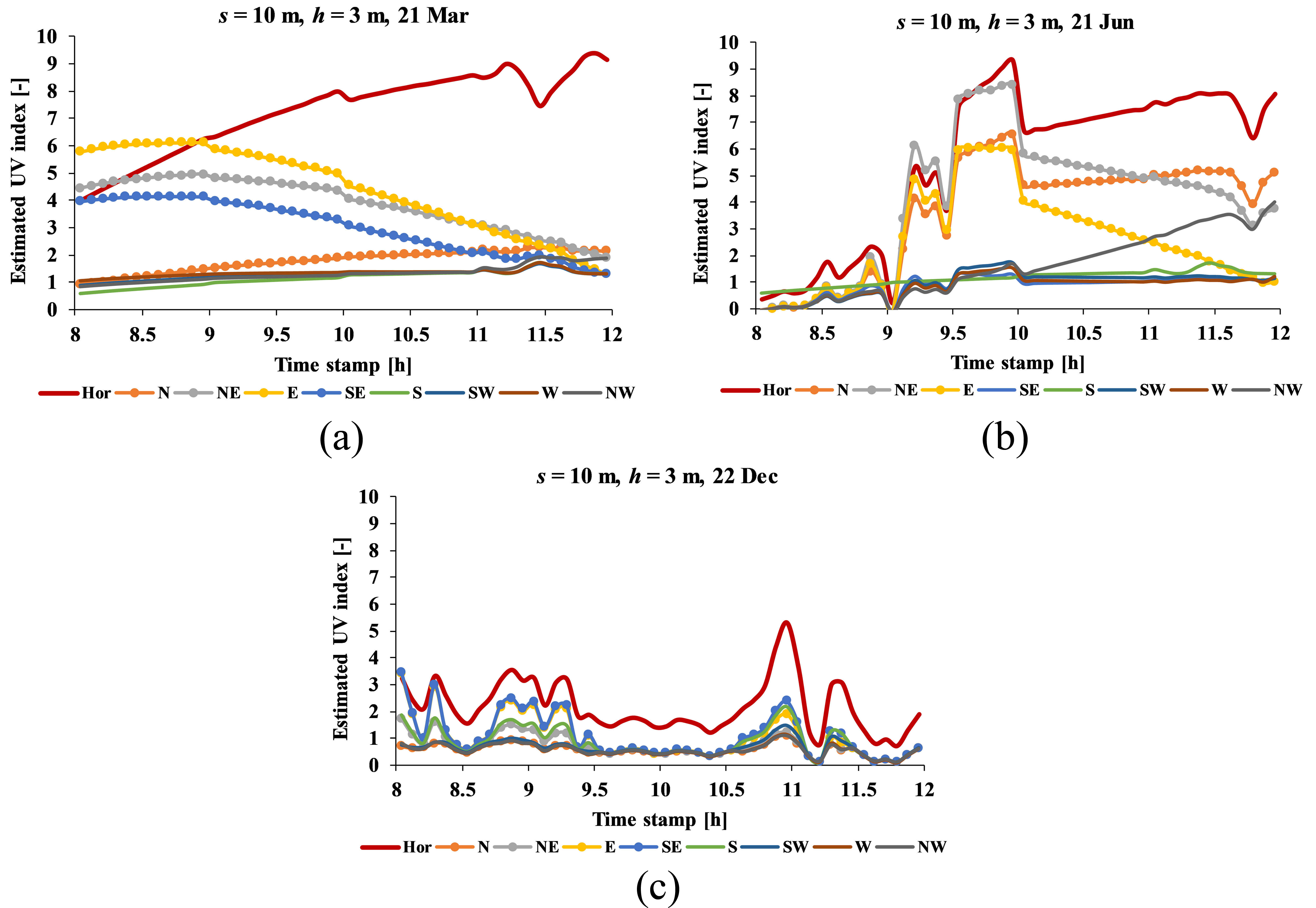
Fig. 12. Estimated UV index within 08.00~12.00 hrs in the courtyard scene with s = 10 m, h = 3 m on (a) 21 March, (b) 21 June, and (c) 22 December.

Figure 13

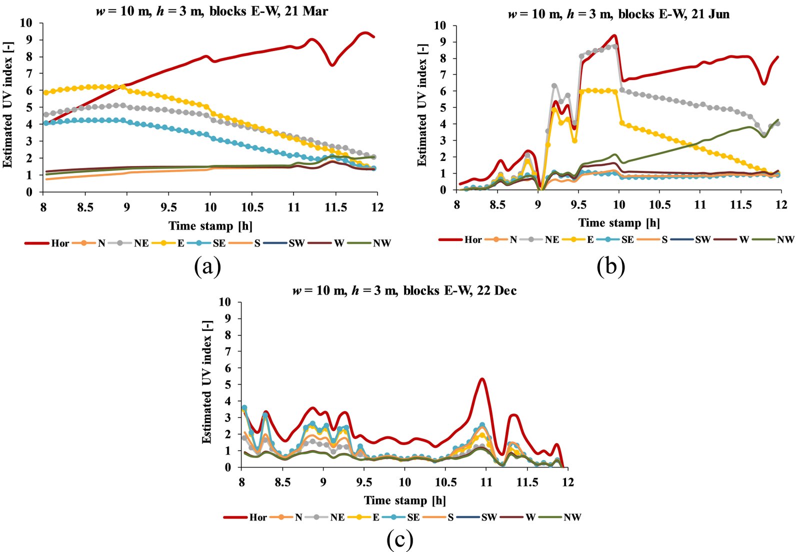
Fig. 13. Estimated UV index within 08.00~12.00 hrs in the street canyon scene with w = 10 m, h = 3 m, blocks in east and west on (a) 21 March, (b) 21 June, and (c) 22 December.

The daily profiles in Figs. 12 and 13 are arguably similar with that of the baseline scene (Fig. 8). Comparison with Table 3 also suggests that the peak UVI values depicted in both figures are about one scale lower than those in the baseline scene. On 21 March, the horizontal UVI is 9 (very high risk) at few minutes before 12.00 hrs, and the maximum vertical UVI is 6 (high risk) at around 09.00 hrs, facing east. On 21 June, the peak time is between 09.30 and 10.00 hrs with UVI 9, achieved on the horizontal and northeast-facing planes. On 22 December, the UVI on all planes are relatively low, and so the effect of orientation on vertical UVI is also small. The peak time for horizontal plane (UVI 5, moderate risk) on this day is at around 11.00 hrs, but the peak time for vertical planes is achieved when facing southeast (UVI 3~4, moderate risk) at around 08.00 hrs.

Generally, in the scenarios with 3-m high building blocks, the maximum daily horizontal UVI is estimated to vary from 5, in typical overcast days in December, up to 9, in days with intermediate sky in March~June. While the maximum horizontal UVI in March and June are relatively similar, the maximum UVI on vertical planes are different. In the courtyard scene with s = 10 m and h = 3 m, on 21 March, the maximum vertical UVI is 6, facing east; on 21 June it is 8, northeast; whereas on 22 December it is 3, southeast. In the street canyon scene with w = 10 m, h = 3 m, and east-west building blocks, the maximum vertical UVI on the three days are respectively 6, facing east; 9, northeast, and 4, southeast. The peak time stamps for the street canyon scenes are mostly the same with those for the courtyard. Again, these are valid in the scenarios with 3-m high building blocks. In courtyards or streets surrounded with higher blocks, the estimated UVI would become lower, and so would also the risk.

It should be noticed that the sun’s relative position in the end of the year is above the southern hemisphere, thus the southeast-facing plane shall receive more sunlight exposure compared to the northeast-facing one. The opposite is true in the middle of the year, in which the northeast-facing plane will get more sunlight exposure. The amount of surface irradiance, and thus the UVI, on the northeast-facing plane on 21 June however would be greater than that on the southeast-facing plane on 22 December, due to lesser amount of daily rainfalls and cloud cover in the former situation compared to the latter.

To summarise, as far as the vertical planes are concerned, in the urban context with 3-m high surrounding buildings in the city of Bandung, care should be primarily taken on 21 June (or any day with similar daily profile), due to very high risk of UV radiation (UVI 8~9) at around 09.30~10.00 hrs when facing northeast. On 21 March, the maximum UVI is 6 (high risk) at around 09.00 hrs when facing east. The typical day of 22 December is the one with the least concern, since the maximum UVI is only 3~4 (moderate), achieved at around 08.00 hrs when facing southeast. At any different time stamp within 08.00~12.00 hrs and when facing other orientations, the UVI values shall be lower and hence also the risk.

As mentioned in Subsection 2.3, the measurements of UVI and daily horizontal E_e,g were conducted in the rooftop of Labtek IXB Building in ITB Campus in Bandung. Although conducted in the rooftop, there are also neighbouring buildings with the same or larger height, so the measurement site is not completely unobstructed, i.e. it also captures reflections from the surroundings. In the model, as mentioned in Subsection 2.1, the building blocks is set to have a spectrally neutral reflectance of 0.5, i.e. the Radiance material is modelled to have the red, green, and blue (RGB) reflectance values of (0.5, 0.5, 0.5).

To verify whether the spectral reflectance components may significantly influence the obtained UVI values, two modelled scenarios are revisited. These are the courtyard scene with s = 5 m, h = 9 m; and the street canyon scene with w = 5 m, h = 9 m, building blocks at east-west. In both scenes, the Radiance RGB reflectance values are changed to (0.62, 0.5, 0) and then to (0, 0.65, 1). Both combinations correlate to the spectrally-weighted (average) reflectance of 0.5, according to the JALOXA Colour Picker online tool [40]. While the average reflectance remains the same with the original, the visual appearance will undoubtedly be different; the former combination appears light brown, while the latter appears light blue. Both combinations are also the most ‘extreme’ one can have while maintaining the average reflectance of 0.5, to enable comparison with the original scene.

Simulations in Daysim are again conducted, followed with the necessary conversion, to obtain the daily maximum UVI values on horizontal and vertical planes. The results for all time stamps within the entire year are compared with those obtained from the original scene. The root-mean-square deviation (RMSD) between the modified and the original scene values are reported in Table 6.

Table 6

Root-mean-square deviation (RMSD) of the daily maximum UVI values on horizontal and vertical planes due to various RGB reflectance values of the building blocks as compared to the original scene.

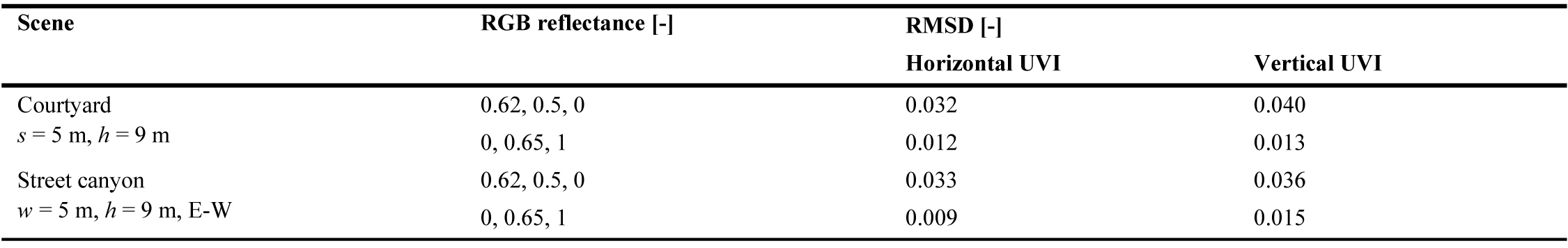
Table 6. Root-mean-square deviation (RMSD) of the daily maximum UVI values on horizontal and vertical planes due to various RGB reflectance values of the building blocks as compared to the original scene.

It is observed that the RMSD in all scenes, considering all days in the entire year, are never greater than 0.04. The change of spectral reflectance components (while maintaining the spectrally-weighted average), even in the most extreme case, slightly changes the global irradiance and the corresponding UVI values. Nevertheless, the differences are very subtle and practically insignificant in changing the UVI values of the original scenes.

3.3. Sensitivity analysis

Tables 7 and 8 report the standard regression coefficient (SRC) values of the relevant input parameters respectively for the courtyard and street canyon scene, with regard to the daily maximum estimated horizontal and vertical UVI. The SRC values are based on the analysis involving only the three selected days (21 March, 21 June, and 22 December) and involving the entire 365 days in a year. The adjusted R² values (R²_adj) are also reported in both tables.

Table 7

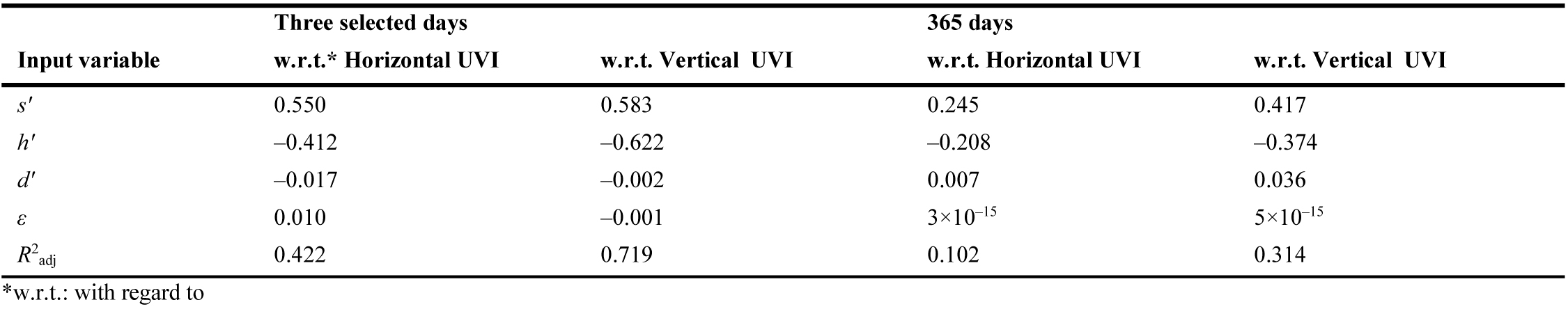
Standard regression coefficient (SRC) values of the relevant input parameters for the courtyard scene, for the three selected days and for the entire year, with regard to the estimated horizontal and vertical UVI.

Table 7. Standard regression coefficient (SRC) values of the relevant input parameters for the courtyard scene, for the three selected days and for the entire year, with regard to the estimated horizontal and vertical UVI.

Table 8

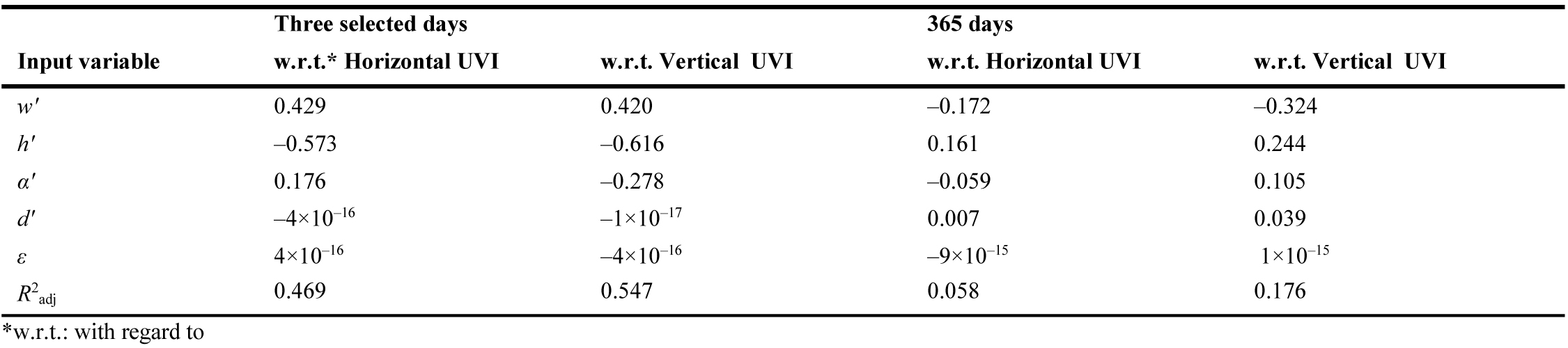
Standard regression coefficient (SRC) values of the relevant input parameters for the street canyon scene, for the three selected days and for the entire year, with regard to the estimated horizontal and vertical UVI.

Table 8. Standard regression coefficient (SRC) values of the relevant input parameters for the street canyon scene, for the three selected days and for the entire year, with regard to the estimated horizontal and vertical UVI.

It is observed that for the courtyard scene, the highest R²_adj (0.719), and thus is the most reliable, is achieved for the model involving daily maximum vertical UVI evaluated for the three selected days. In that model, the most influential input parameter is the building height (SRC = –0.622), followed with the courtyard size (SRC = 0.583). This means as the surrounding buildings get higher, the daily maximum vertical UVI becomes lower, as expected. Also, when the courtyard size is larger, the daily maximum vertical UVI becomes higher due to less shading effect. The impact of days is generally negligible (SRC ≈ 0), i.e. regardless of the day, the change of daily maximum estimated UVI is not statistically significant.

With regard to the horizontal UVI for the three selected days, the most influential input parameter is found to be the courtyard size (SRC = 0.550), followed with the building height (SRC = –0.412). However, the R²_adj of the model is 0.422, meaning that the proposed model can only explain less than 50% of the input-output relationship. The full annual sensitivity analysis gives even smaller R²_adj values, and is therefore less reliable than the three-day sensitivity analysis.

For the street canyon scene, the highest R²_adj (0.547) is also achieved for the model involving daily maximum vertical UVI evaluated for the three selected days. In that model, the most influential input parameter is the building height (SRC = –0.616), followed with the street width (SRC = 0.420). The impact of building blocks’ orientation is rather small (SRC = –0.278). This suggests that large values of maximum vertical UVI can be achieved in situations with low building height or wide street canyon, regardless the orientation and day of the year.

With regard to the horizontal UVI for the three selected days, the most influential input parameter is found to be the building height (SRC = –0.573), followed with the street width (SRC = 0.429). As in the courtyard scenario, the full annual sensitivity analysis for the street canyon scene also gives small R²_adj values, and so the results are therefore less reliable than those from the three-day sensitivity analysis.

It is to be noticed that the sensitivity analysis in this study is conducted to systematically determine the influence of the input parameters of the surrounding buildings on the estimated UVI. It is not specifically conducted to find the best-fitted model itself. Therefore, only the multiple linear regression model is considered in this case, because it is the most commonly employed model in sensitivity analysis.

In addition, while most of the obtained R²_adj values in the sensitivity analysis are rather small, the values with regard to the vertical UVI on the three selected days are greater than 0.5. For the courtyard scene, the R²_adj is relatively high (0.719) and is thus quite reliable given the high variability of the obtained data. Nevertheless, developing a best-fitted model can be considered in the extension of the study in the future.

In general, the results in Tables 7 and 8 suggest that sensitivity analyses for the three selected days are more reliable compared to those for the entire year. In other words, there are significant differences between the daily maximum UVI on the three days of solstices and equinox. Meanwhile, when all days in a year are considered, the differences between daily maximum UVI values are less significant, and thus no strong correlations can be constructed. This is somewhat expected since the site is located in the tropics, where seasonal variations are little and perhaps insignificant. Moreover, the influence of the building parameters on the vertical UVI is generally higher than that on the horizontal UVI. It should be noted however that the vertical UVI values considered in this analysis are the maximum among all eight orientations, i.e. the values do not represent only a single orientation, as reported in Subsection 3.2.

4. Discussion

Few remarks can be mentioned regarding the presented study. First of all, the modelled site is in located in the tropical climate zone, but is also at a high altitude of about 750 m above sea level. Most Indonesian large cities are however located in or around the coast area, thus the microclimate can be different, e.g. the annual mean temperature is generally higher. Sites at high altitude are however prone to high amount of solar radiation, which justifies the motivation of this study.

The entire findings in this case are based on the provided daylighting profiles in the EPW data file, which combines data from various years. As mentioned in Subsection 2.1, the associated data file is a typical meteorological year (TMY), in which data for different months are extracted from different years within the years 1997~2004, based on continuous measurements at the on-site weather monitoring station at the Institute of Research and Development for Dwellings in Bandung. Thus, the reported results for a given day may not exactly represent the actual condition under the same day. For instance, the results for 21 March may be different compared to those obtained on an actual day of 21 March (either in the past or in the future) that has a largely different daily profile, despite being in the same location. Conversely, it may be well representative for other days in March, as long as the daily profile is similar (see Subsection 3.1.1). In any case, climate data are mostly statistical summaries of the past situations, while the climate itself is constantly changing. Therefore, any prediction or forecast based on such data will always contain errors relative to the actual situation.

Nevertheless, the proposed models in Eqs. (7) or (8) can be applied to estimate the instantaneous UVI at a given time in or around the city of Bandung, as long as the E_v,g is known. Again, this will not be entirely free from errors; but since the UVI is typically reported as integers, the proposed models are expected to be sufficient as the first estimation.

The global illuminance E_v,g near the ground or street level shall be easily measured using an affordable illuminance-meter with a broad measurement range (e.g. up to 100 000 lx), provided the instrument is calibrated and conforms to recognised standards. Based on the estimated UVI value, one can estimate whether it is safe enough to expose oneself to outdoor daylight in the relevant scenes (with surrounding buildings) at that particular time; and if so, which vertical orientation shall be preferred.

It is indeed possible in Daysim to directly estimate the irradiance values by setting the sensors to measure irradiance instead of illuminance. Reinhart [41] also mentioned that “the Daysim program ds_illum has a luminous efficacy model according of Perez built-in that converts irradiance into illuminances if you choose the latter type of output. Otherwise, Daysim just uses the direct and diffuse irradiances for an EPW weather file.”. In other words, the method applied in this current study also follows the same method as what Daysim does in the direct conversion between irradiance and illuminance, only with a more elaborative way.

There are also other advantages of using illuminance instead of irradiance in this case. In contrast, a handheld instrument to measure solar irradiance is perhaps less affordable for laypeople. Also, most building designers and practitioners are reasonably familiar with the use of illuminance, since it is mentioned in building standards and codes on (day)lighting. One can thus relate the obtained E_v,g values can with the indoor lighting performance at the same time, which may also indirectly influence the building design process. Therefore, the E_v,g data are nonetheless presented in this study.

The influence of surrounding buildings on the E_v,g are represented in their daily profiles, instead of the numerical values themselves, because the values greatly vary throughout the year and are not formally standardised against a certain criterion. In contrast, numerical values of the maximum UVI are of more interest because the values themselves can be compared with the reference and have a direct risk on human health.

As far as simulation is concerned, the choice of surrounding buildings typology may also influence the outcomes. In this study, the building blocks are set to have a certain equal height; while in reality, the heights are not uniform and so the resulting shading effect will become more complicated. Surface reflectance of the blocks may also be influential; the value in this study is set constant at 0.5, which represents the middle value for actual building exterior surface [25], but it can differ in reality. The reflectance is also almost certainly not uniform, because the exterior building walls may consist of various surface finishing. Smaller surface reflectance shall result in more shades and thus can lower the risk of UV overexposure, but it can also reduce the health advantage regarding vitamin D. Greater surface reflectance shall do the opposite, and so more care should be taken to ensure the sunbathing activity is done within the optimum time stamp and duration.

With regard to optimum duration, no specific recommendations are explicitly given in this study, since there are other factors to consider, while cannot simply be simulated. It is understood nonetheless that the recommended duration of sunlight exposure is related not only with the UVI, but also with the human skin colour type [42,43] and the applied solar protection. In general, people with lighter skin colour may be exposed to sunlight in a shorter duration, compared to those with darker skin colour, before their skin become tanned and/or burnt. Several online calculators (e.g. [44-46]) are nowadays available to estimate the maximum duration of sunlight exposure, for any skin colour type under a given UVI.

Despite the limitations, this current study thus has the main contribution in providing the relevant UVI under various outdoor scenarios with surrounding buildings, particularly in the tropical region. Even though the simulation is performed using climate data for only a particular location in the tropics, the proposed methodology is expected to be applicable for other locations and regions in the world, which hopefully can help in promoting good practice of healthy activities in the society.

5. Conclusions

This study has demonstrated the capability of annual daylighting simulation to estimate the impact of courtyard and street canyon to the peak time and values of global horizontal and vertical illuminances (E_v_,g) at a point 1.5 m above the ground in the tropical city of Bandung, Indonesia. Simulations are performed for the time frame of 08.00~12.00 hrs during the whole year, representing the sunbathing activity in the morning. The impact of such surrounding buildings on the E_v_,g daily profiles and the estimated ultraviolet index (UVI) has been also reported. The instantaneous UVI at peak times in the particular location can be estimated from the corresponding E_v_,g at the same time, according to the proposed linear model: UVI ≈ 8.89 × 10^–5 E_v_,g – 0.42, which can be useful to perform conversion between both variables whenever necessary.

Simulations of the courtyard scenes suggest that in the case of building blocks height h = 3 m, the UVI reduction due to shading effect is subtle, and thus having higher risk of UV radiation, except for the courtyard size s = 5 m. Overall, the highest risk would be achieved when s = 10 m and h = 3 m, where the maximum horizontal UVI on 21 March, 21 June, and 22 December are respectively 9 (very high risk), at around 12.00 hrs; 9 (very high risk), at 10.00 hrs; and 5 (moderate risk), at 11.00 hrs. The corresponding, maximum vertical UVI on those days are: 6 (high risk), facing east at 09.00 hrs; 8 (very high risk), facing northeast at 10.00 hrs; and 3 (moderate risk), facing southeast at 08.00 hrs.

Simulations of the street canyon scenes suggest that the 5-m wide street is more sensitive to height variation, compared to the 10-m wide. The impact of orientation on the vertical UVI is little when the street is narrow and the surrounding blocks are high (w = 5 m and h = 9 m), in which the peak is achieved at 11.00 hrs. In all 10-m wide street scenarios, the maximum vertical UVI are achieved when facing east. Overall, the highest risk would be achieved when w = 10 m, h = 3 m, with east-west building blocks (i.e. north-south street direction). Daily profiles for that scenario on 21 March, 21 June, and 22 December suggests that the maximum horizontal UVI are respectively 10 (very high risk), at around 12.00 hrs; 9 (very high risk), at 10.00 hrs; and 5 (moderate risk), at 11.00 hrs. The corresponding, maximum vertical UVI on those days are: 6 (high risk), facing east at 09.00 hrs; 9 (very high risk), facing northeast at 10.00 hrs; and 4 (moderate risk), facing southeast at 08.00 hrs.

Multiple linear regressions with regard to daily maximum estimated UVI for the courtyard scene show that the most reliable model (R²_adj = 0.719) is the daily maximum vertical UVI evaluated for the three selected days. In that model, the most influential input parameter is the building height (SRC = –0.622), followed with the courtyard size (SRC = 0.583). The impact of days is generally negligible. For the street canyon scene, the most reliable model (R²_adj = 0.547) also involves daily maximum vertical UVI evaluated for the three selected days, where the most influential input parameter is the building height (SRC = –0.616), followed with the street width (SRC = 0.420). The full annual sensitivity analysis gives small R²_adj values, and so the results are less reliable than those obtained from the three-day sensitivity analysis.

Acknowledgement

This research is supported by the Ministry of Research and Technology of the Republic of Indonesia, under the Fundamental Research (PDUPT) scheme, with the contract number 2/E1/KP.PTNBH/2020.

Contributions

R. A. M. designed the research framework, performed the simulation, and wrote the manuscript. M. D. K. executed the measurement and co-wrote the manuscript. B. P. provided the instrumentation and co-wrote the manuscript.

Declaration of competing interest

The authors report no conflicts of interest. The authors alone are responsible for the content and writing of this article.

References

B.A. Ingraham, B. Bragdon, A. Nohe, Molecular basis of the potential of vitamin D to prevent cancer, Current Medical Research Opinion 24 (2008) 139–149. https://doi.org/10.1185/030079907x253519
D.D. Bikle, Protective actions of vitamin D in UVB induced skin cancer, Photochemistry and Photobiological Science 11 (2012) 1808–1816. https://doi.org/10.1039/c2pp25251a
C. Gordon-Thomson, R. Gupta, W. Tongkao-on, A. Ryan, G.M. Halliday, R. S. Mason, 1a,25 dihydroxyvitamin D3 enhances cellular defenses against UV-induced oxidative and other forms of DNA damage in skin, Photochemistry and Photobiological Science 11 (2012) 1837–1847. https://doi.org/10.1039/c2pp25202c
A. Hossein-Nezhad, M.F. Holick, Vitamin D for health: A global perspective. Mayo Clinical Proceedings 88 (2013) 720–755. https://doi.org/10.1016/j.mayocp.2013.05.011
A.A. Silva, Improving photoprotection attitudes in the tropics: Sunburn vs vitamin D, Photochemistry and Photobiology 90 (2014) 1446–1454. https://doi.org/10.1111/php.12347
World Health Organization (WHO), Ultraviolet Radiation, EHC 160, World Health Organization, Geneva, 1994.
D. Cano, J.M. Monget, M. Albuisson, H. Guillard, N. Regas, L. Wald, A method for the determination of the global solar radiation from meteorological satellite data, Solar Energy 37 (1986) 31–39. https://doi.org/10.1016/0038-092x(86)90104-0
Commission Internationale de l’Éclairage (CIE), CIE 108:1994: Guide to Recommended Practice of Daylight Measurement. CIE Central Bureau, Vienna, 1994. https://doi.org/10.1002/col.5080200118
International Energy Agency (IEA), IEA-SHCP-17E-2: Broad-band visible radiation data acquisition and analysis. A technical report of task 17: measuring and modelling spectral radiation affecting solar systems and buildings, vol. 2. Satellite Report No. 1 World Network of Daylight Measuring Stations (IDMP), ASRC Albany, N.Y, 1994.
R.A. Mangkuto, M. Rohmah, A.D. Asri, Design optimisation for window size, orientation, and wall reflectance with regard to various daylight metrics and lighting energy demand: A case study of buildings in the tropics, Applied Energy 164 (2016) 211–219. https://doi.org/10.1016/j.apenergy.2015.11.046
R.A. Mangkuto, M.A.A. Siregar, A. Handina, Faridah, Determination of appropriate metrics for indicating indoor daylight availability and lighting energy demand using genetic algorithm, Solar Energy 170 (2018) 1074–1086. https://doi.org/10.1016/j.solener.2018.06.025
R.A. Mangkuto, A.P. Rachman, A.G. Aulia, A.D. Asri, M. Rohmah, Assessment of pitch floodlighting and glare condition in the Main Stadium of Gelora Bung Karno, Indonesia, Measurement 117 (2018) 186–199. https://doi.org/10.1016/j.measurement.2017.12.016
N. Farida, Effects of outdoor shared space on social interaction in a housing estate in Algeria, Frontiers of Architectural Research 2 (2013) 457–467. https://doi.org/10.1016/j.foar.2013.09.002
N. Jang, S. Ham, A study on courtyard apartment types in South Korea from the 1960s to 1970s, Frontiers of Architectural Research 6 (2017) 149–156. https://doi.org/10.1016/j.foar.2017.03.004
P. Moonen, T. Defraeye, V. Dorer, B. Blocken, J. Carmeliet, Urban Physics: Effect of the micro-climate on comfort, health and energy demand, Frontiers of Architectural Research 1 (2012) 197–228. https://doi.org/10.1016/j.foar.2012.05.002
Á. Szűcs, Wind comfort in a public urban space—Case study within Dublin Docklands, Frontiers of Architectural Research 2 (2013) 50–66. https://doi.org/10.1016/j.foar.2012.12.002
C.F. Reinhart, S. Herkel, S., The simulation of annual daylight illuminance distributions – a state-of-the-art comparison of six RADIANCE-based methods, Energy and Buildings 32 (2000) 167–187. https://doi.org/10.1016/s0378-7788(00)00042-6
C.F. Reinhart, O. Walkenhorst, Validation of dynamic RADIANCE-based daylight simulations for a test office with external blinds, Energy and Buildings 33 (2001) 683–697. https://doi.org/10.1016/s0378-7788(01)00058-5
O. Walkenhorst, J. Luther, C.F. Reinhart, J. Timmer, Dynamic annual daylight simulations based on one-hour and one-minute means of irradiance data, Solar Energy 72 (2002) 385–395. https://doi.org/10.1016/s0038-092x(02)00019-1
MIT Sustainable Design Lab, DAYSIM, 2020. Available online at: https://github.com/MITSustainableDesignLab/Daysim.
R. Perez, P. Ineichen, R. Seals, J. Michalsky, R. Stewart, Modeling daylight availability and irradiance components from direct and global irradiance, Solar Energy 44 (1990) 271–289. https://doi.org/10.1016/0038-092x(90)90055-h
R. Perez, R. Seals, J. Michalsky, All-weather model for sky luminance distribution — preliminary configuration and validation, Solar Energy 50 (1993) 235–245. https://doi.org/10.1016/0038-092x(93)90017-i
Badan Standardisasi Nasional (BSN), SNI T-14-2004: Geometri Jalan Perkotaan, BSN, Jakarta, 2004. [in Indonesian: SNI T-14-2004: Urban Road Geomertry]
American Association of State Highway Transportation Officials (AASHTO), A Policy on Geometric Design of Highways and Streets, 7th ed., AASHTO, Washington, DC, 2018.
S.A. Venegas Quintulén, M.B. Piderit Moreno, Reflectancia de las envolventes verticales y su influencia sobre disponibilidad de luz natural en el cañón urbano de la ciudad de Concepción, Revista Hábitat Sustentable 8 (2018) 6–15. https://doi.org/10.22320/07190700.2018.08.01.01
A.H. Fakra, B. Boyer, F. Miranville, D. Bigot, A simple evaluation of global and diffuse luminous efficacy for all sky conditions in tropical and humid climate, Renewable Energy 36 (2011) 298-306. https://doi.org/10.1016/j.renene.2010.06.042
P. Chaiwiwatworakul, S. Chirarattananon, Luminous efficacies of global and diffuse horizontal irradiances in a tropical region, Renewable Energy 53 (2013) 148–158. https://doi.org/10.1016/j.renene.2012.10.059
M. Allaart, M. van Weele, P. Fortuin, H. Kelder, An empirical model to predict the UV-index based on solar zenith angles and total ozone, Meteorological Application 11 (2004) 59–64. https://doi.org/10.1017/s1350482703001130
V. Fioletov, J.B. Kerr, A. Fergusson, The UV index: Definition, distribution and factors affecting it, Canadian Journal of Public Health 101 (2010), I5–I9. https://doi.org/10.1007/bf03405303
P. Moshammer, S. Simic, D. Haluza, UV “indices” – What do they indicate?, International Journal of Environmental Research on Public Health 13 (2016) 1041. https://doi.org/10.3390/ijerph13101041
Commission Internationale de l’Éclairage (CIE), Rationalizing nomenclature for UV doses and effects on humans, Technical Report, Joint publication of CIE and WMO (World Meteorological Organization), CIE 209:2014 – WMO/GAW Report No. 211, 2014.
K.A. Tereszchuk, Y.J. Rochon, C.A. McLinden, P.A. Vaillancourt, Optimizing UV Index determination from broadband irradiances. Geoscience Model Development 11 (2018) 1093–1113. https://doi.org/10.5194/gmd-11-1093-2018
A.F. McKinlay, B.L. Diffey, A reference action spectrum for ultraviolet induced erythema in human skin. CIE Research Note, 6, 17–22, 1987.
A.R. Webb, H. Slaper, P. Koepke, A.W. Schmalwieser, Know your standard: Clarifying the CIE erythema action spectrum. Photochemistry and Photobiology 87 (2011) 483–486. https://doi.org/10.1111/j.1751-1097.2010.00871.x
World Meteorological Organization (WMO), Report on the WMO Meeting of Experts on UV-B Measurements, Data Quality and Standardization of UV Indices, WMO/TD-No. 625, 1995.
World Health Organization (WHO), Global Solar UV Index: A Practical Guide, World Health Organization, Geneva, 2002.
Ambient Weather, Dashboard (AR ITB 1), 2020. Available online at: https://ambientweather.net/dashboard/6c5794c59bfeeb1a4f05945bc618fa80.
R. Rahim, Baharuddin, R. Mulyadi, Classification of daylight and radiation data into three sky conditions by cloud ratio and sunshine duration, Energy and Buildings 36 (2004) 660–666. https://doi.org/10.1016/j.enbuild.2004.01.012
R. Rahim, Teori dan Aplikasi Distribusi Luminansi Langit di Indonesia, Universitas Hasanuddin, Makassar, 2009. [in Indonesian: Theory and Application of Sky Luminance Distribution in Indonesia]
JALOXA, Colour Picker, 2013. Available online at: https://www.jaloxa.eu/resources/radiance/colour_picker/index.shtml.
C.F. Reinhart, [Radiance-daysim] Calculation of the solar irradiation with Daysim, in: Radiance-daysim mailing list, 2016. Available online at: https://www.radiance-online.org/pipermail/radiance-daysim/2016-August/000125.html.
T.B. Fitzpatrick, The validity and practicality of sun-reactive skin types I through VI, Archives of Dermatology 124 (1988) 869–871. https://doi.org/10.1001/archderm.124.6.869
A.R. Webb, O. Engelsen, Calculated ultraviolet exposure levels for a healthy vitamin D status, Photochemistry and Photobiology 82 (2006) 1697–1703. https://doi.org/10.1562/2006-09-01-ra-670
United States Environmental Protection Agency (EPA), UV Index, 2019. Available online at: https://www.epa.gov/sunsafety/uv-index-1.
AnyCalculator, Kim’s Sun Tanning Calculator, 2020. Available online at: http://www.anycalculator.com/tanningcalculator.html.
M. Koperska, Sunbathing calculator, 2020. Available online at: https://www.omnicalculator.com/other/sunscreen.

Get PDF (14.2 MB)

SHARE ON