Volume 7 Issue 2 pp. 222-237 • doi: 10.15627/jd.2020.19
A Field-validated Multi-objective Optimization of the Shape and Size of Windows Based on Daylighting Metrics in Hot-summer Mediterranean and Dry Summer Continental Climates
Farzam Kharvari∗
Author affiliations
Society for Research on Education, Design, and Architecture (SEDARCH), Ottawa, Canada
* Corresponding author. F.kharvari@sedarch.com; f.kharvari@gmail.com (F. Kharvari)
History: Received 15 September 2020 | Revised 26 October 2020 | Accepted 29 October 2020 | Published online 11 November 2020
Copyright: © 2020 The Author(s). Published by solarlits.com. This is an open access article under the CC BY license (http://creativecommons.org/licenses/by/4.0/).
Citation: Farzam Kharvari, A Field-validated Multi-objective Optimization of the Shape and Size of Windows Based on Daylighting Metrics in Hot-summer Mediterranean and Dry Summer Continental Climates, Journal of Daylighting 7 (2020) 222-237. https://dx.doi.org/10.15627/jd.2020.19
Figures and tables
Abstract
This study aims to determine the optimum size of windows based on the window-to-floor ratio (WFR) for the main cardinal directions in Hot-summer Mediterranean (Csa) and Dry Summer Continental (Dsa) climates (Köppen–Geiger classification system) by carrying out a multi-objective optimization that relies on three dynamic metrics of Useful Daylight Illuminance (UDI-a (autonomous)), Daylight Autonomy (DA), and Annual Sunlight Exposure (ASE1000,250) in Radiance version 5.1. A validation against field measurements is conducted under an overcast sky with an illuminance of 11000 lux. The Pareto front is used to pick the best solutions for evaluating the most optimized solutions. Accordingly, the minimum standards for cardinal directions in each climate are defined. The minimum suggested WFR for the Dsa and Csa climates for the south-, east-, north-, and west-facing windows are 20%, 15%, 20%, and 15% (Dsa) and 20%, 20%, 25%, and 20% (Csa), respectively. Furthermore, the results show the shape and relative proportions of windows (vertical/horizontal) have a significant effect on the metrics. As a result, this paper introduces the “Proportion Ratio” as a new indicator for designing windows.
Keywords
Multi-objective optimization, Radiance, HoneybeePlus, Field Measurements
1. Introduction
Architects and designers are required to invest a lot of time in making decisions for various aspects of their buildings during the early stages of the design [1,2]. One of the major decisions during this process is determining the size of windows but it is one of the most complex decisions in the early stages of design since there are so many parameters involved [3]. There is extensive literature on the benefits of efficient daylighting. The efficient design of windows contributes to reducing the energy consumption of buildings [4], reducing the need for artificial lighting [2], improving visual and thermal comfort [5,6], improving occupants’ health [7], and enhancing circadian rhythm [8]. However, choosing efficient window sizes is not a simple design problem since various factors are generally involved that can offset each other. For instance, increasing the surface of windows may reduce the need for artificial lighting and heating in winter but may result in excessive energy use in summer. Besides, local and cultural issues make the situation more complex. For instance, the size of windows in an arid climate differs from the Mediterranean climate.
As a result, designing efficient windows is a multifaceted topic and there are many objectives involved in achieving optimum proportions for windows.
As a result, Climate-based Daylight Modeling, known as CBDM [9], has been officially introduced in recent 2006 in which the windows are optimized based on the location of projects. In this approach, dynamic metrics such as the Useful Daylight Illuminance (UDI-a (autonomous)) are used instead of static metrics such as the Daylight Factor (DF) that do not consider local conditions such as sun azimuth or weather conditions. Consequently, these local conditions make the design process more complex.
In recent years, multi-objective optimization has significantly helped architectural projects since it can solve complex problems with various changing parameters and provide the best solutions to a defined problem [3]. While this method is being used in various projects, many local projects such as ordinary residential constructions and public sector buildings are still being built based on conservative approaches to windows without any localization
and improvement in energy consumption. To date, there has been no study on the minimum acceptable proportion of windows based on the WFR and specific climate conditions based on Köppen- Geiger climate classification. This climate classification makes it possible to generalize the results of CBDM since regions in the classifications include almost similar climate conditions. Most previous multi-objective optimization studies rely on energy optimization of buildings which depends significantly on occupants behavior [10], shading devices and slate angles [11], building envelope and orientation [12,13], and the type of windows [14] based on the Window-to-Wall Ratio (WWR) instead of WFR. It is noteworthy to mention that the acceptable range of WWR is 40% according to the ASHRAE 90.1 standard for some specific climate zones [15]. There are specific multi-objective optimization studies that focused on reducing artificial lighting [2,16], and improving daylighting through designing generative facades [17]. Besides, studies on daylighting focused on finding the best orientation among four cardinal directions [18] and dismiss the shape and orientation of windows (vertical/horizontal windows) on surfaces. In a previous study that focused on determining the size of windows based on the WWR, only UDI-a and discomfort hours were used [19]. Although the orientation of envelopes is studied in these studies, the orientation and proportion of windows themselves (vertical/horizontal) is not investigated. Additionally, using the UDI-a alone is not enough in multi-objective optimization since it uses a range of 300 to 3000 lux [20] because a decrease in the UDI-a does not necessarily mean the illuminance level is not enough but rather it may be decreased due to excessive illuminance levels. Therefore, using Daylight Autonomy (DA) [21] that has a threshold of 300 lux can help interpreting the UDI-a since occupants can use preventative behaviors such as closing curtains in presence of excessive lights. Moreover, as focusing on energy consumption may reduce the generalizations of results, Annual Sunlight Exposure (ASE1000,250) is used as a metric that its higher values can cause visual discomfort (glare) or increase cooling loads [21]. Through these
Therefore, the aim of this study is to determine the optimum size of windows based on the window-to-floor ratio (WFR) for the main cardinal directions in Hot-summer Mediterranean (Csa) and Dry Summer Continental (Dsa) climates (Köppen–Geiger classification system) by carrying out a multi-objective optimization that relies on three dynamic metrics of Useful Daylight Illuminance (UDI-a), Daylight Autonomy (DA), and Annual Sunlight Exposure (ASE1000,250) in Radiance version 5.1. This study uses the intelligent optimization algorithm, HypE, along with Radiance. Then, the optimum solutions are selected based on the Pareto front which is mainly used by researchers [18] and interpreted by secondary values such as the minimum height of windows for better views of outside. Furthermore, although Radiance is a validated tool for daylighting simulations against CIE test cases [22], simulations for research projects without either validation or calibration may deviate significantly from reality [23]. As a result, the simulation model of this study is validated against field measurements prior to conducting the study to make sure that reflectance factors and the model match the reality. In the end, this study suggests minimum percentages for the WFR to achieve efficient daylighting. An advantage of the WFR is its ability to correspond to the depth of penetration of light. Furthermore, this study introduces the “Proportion Ratio” as a new indicator for designing efficient windows in buildings. The outcome of this research can help designers to design efficient windows in the Dsa and Csa climates. The results also establish the foundation for future research on other climates since studies based on climate classification that can be generalized are scarce.
1. Purposes of the work
The purpose of the work is as follows:
- Determining the most optimum solutions for efficient daylighting
- Determining the shape and orientation of windows
- Introducing the optimum height to length ratio of windows as a new indicator named “Proportion Ratio”
- Suggesting minimum required WFRs for incorporation in building codes
2. Methods
This study uses Radiance version 5.1 (hereafter Radiance), a validated program against CIE test cases [22,24], in HoneybeePlus version 0.0.04 and Ladybug version 0.0.68 [25] in Rhino version 6 [26]. An annual grid analysis is used for comparing annual available illuminance levels on the work plane at the height of 76 cm from the ground [27]. The multi-objective optimization is carried out in Octopus version 0.4, a multi-objective optimization interface plugin for Rhino [28], that uses the HypE which was developed based on the HypE for alleviating the hypervolume degeneration problem of NSGA-II [29,30]. It is broadly used by researchers for multi-objective optimizations in buildings [19], [31–33]. Figure 1 shows the research method and outcomes briefly. The next subsections describe the validation and optimizations models (Section 2.1), field data collection for validation (Section 2.2), simulation program and simulation parameters (Section 2.3), dynamic metrics that are used for optimization (Section 2.4), and a short description of HypE/NSGA-II and the Pareto approach for picking the best solutions (Section 2.5).
Figure 1
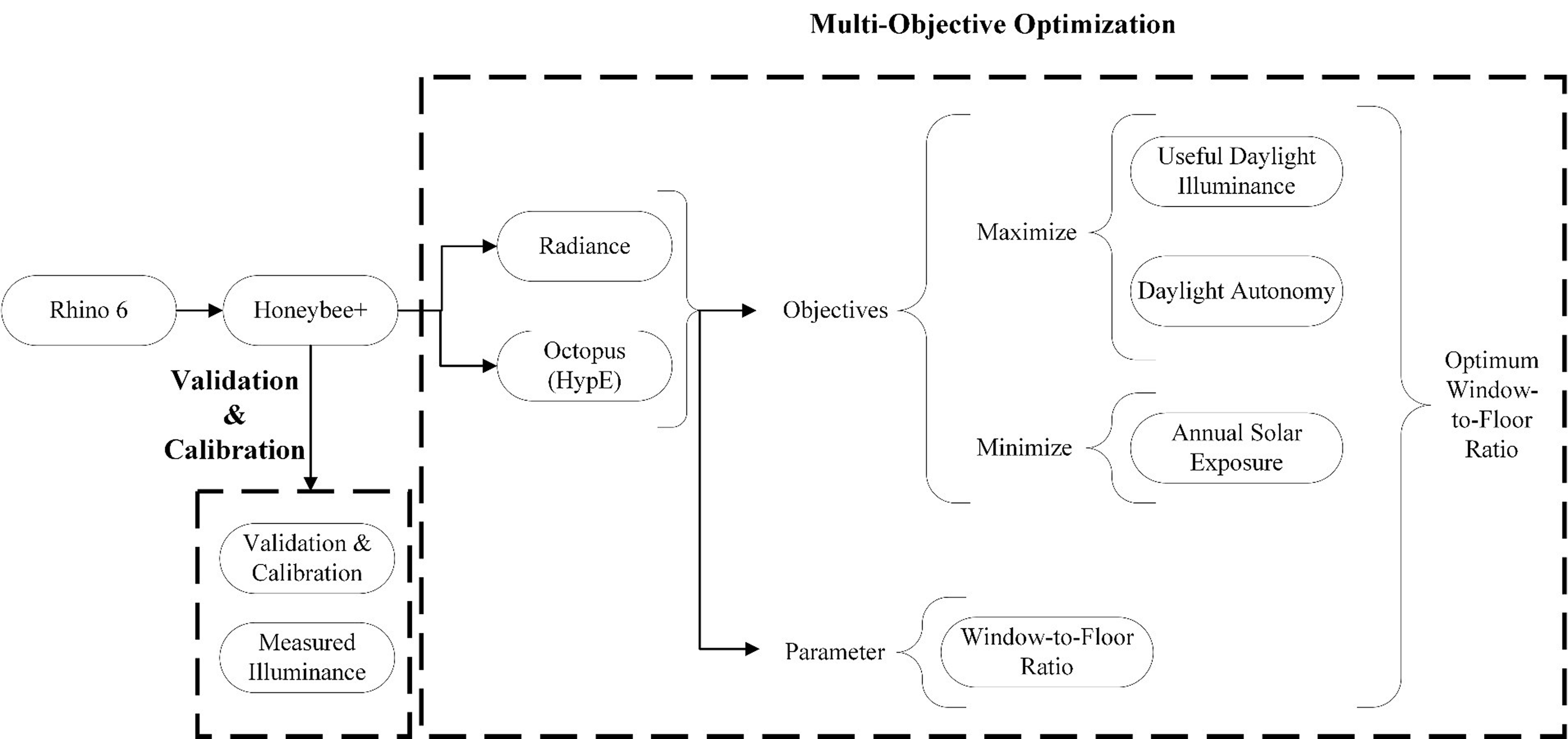
Fig. 1. Research method in brief.
2.1. Simulation model, validation room, and climates
Figure 2 shows the model for validation and multi-objective optimization studies. A base model of 12 m2, which is considered by many standard books as a minimum for main living spaces or offices [34], was used in this study since most cubicles and rooms are having the same size (minimum standard size of living spaces). In addition, this base model omits the effect of depth of penetration in daylighting.
Figure 2
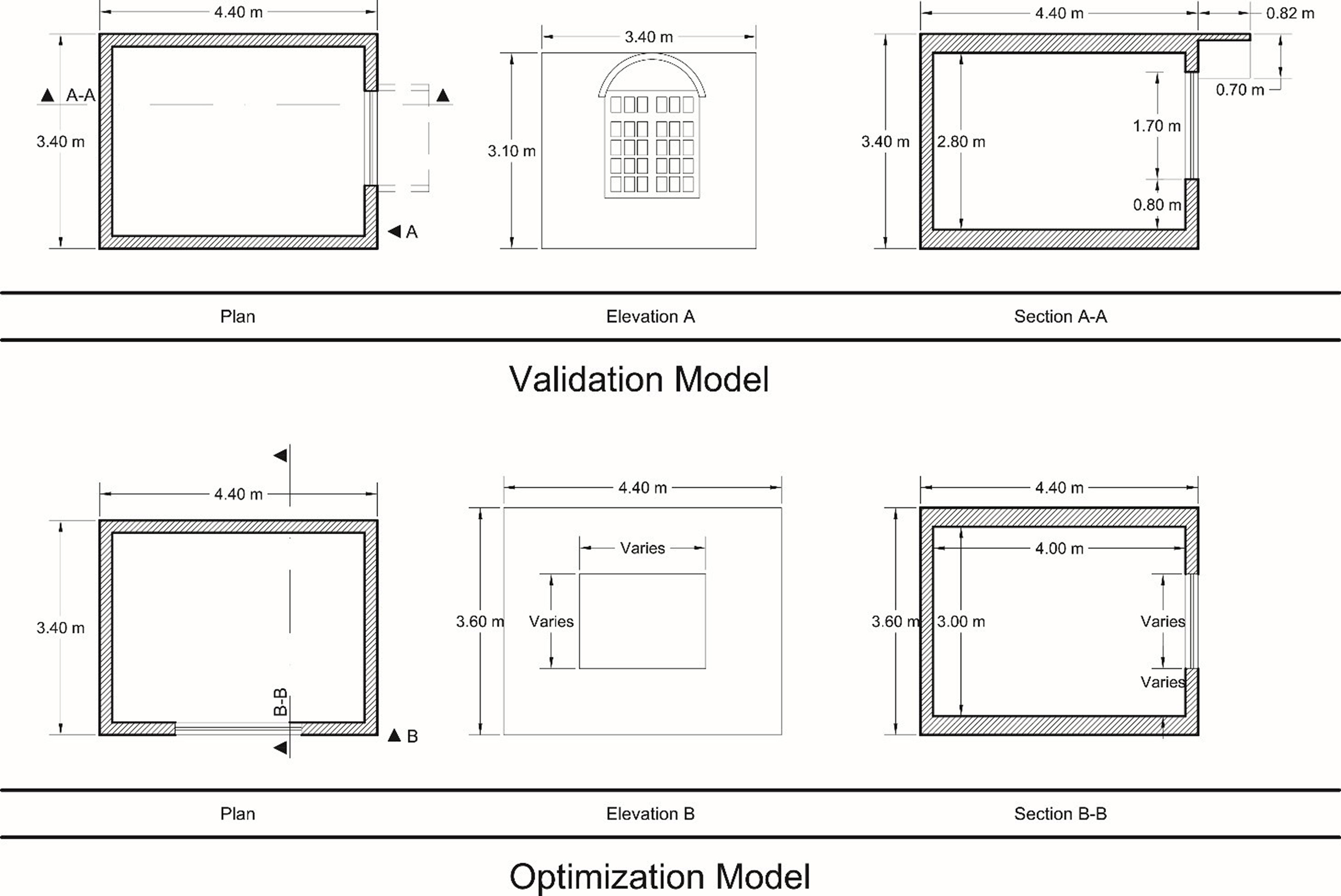
Fig. 2. The interior dimensions of the validation and optimization models..
The optimization model was placed 3 meters above the ground floor and included the environment. The overall reflectance factor for the environment is mentioned in Section 2.3.2. The climate profiles for studies are two cities of Sanandaj (the Dsa climate) and Los Angeles (the Csa climate). The cities are located at 35.3219° N, 46.9862° E (Solar azimuth = 66.68 – 12:00:00 - June 21, 2020) and 34.0522° N, 118.2437° W (Solar azimuth = 91.81 – 12:00:00 - June 21, 2020), respectively.
2.2. Field data collection for validation
This study used the general guidelines of the Illuminating Engineering Society of North America (IESNA) for measuring illuminance levels in indoor environments [27]. The room for validation and calibration was divided into 35 rectangles. Milwaukee MW700 Standard Portable Lux Meter with an accuracy of ±6% of reading/±1 digit [35] was used for measuring the illuminance. The plane for measuring the illuminance level is 760 mm above the floor [27]. Equation 1 shows the general formula for the average illuminance in interior spaces. Respectively, Equation 2 shows the formula for calculating the average illuminance in the studied room in this study. ΣP represents the reading on the measurement points while ΣnPi shows the total number of points. Furthermore, the sky illuminance was measured under an overcast sky with an illuminance level of 11000 lux on November 19, 2019. For modeling purposes, a standard sky with certain illuminance was used which is different from the overcast sky of CIE.
Average Illuminance can be calculated as
Average illuminance in this study is
2.3. Simulation program, simulation parameters, and validation
2.3.1. Simulation program and validation
Radiance version 5.1 is used in this study for analyzing dynamic metrics annually. The model was developed in Rhino version 6 along with HoneybeePlus version 0.0.04 [25] as the interfaces for conducting annual studies in Radiance. Radiance is the calculation engine for lighting in HoneybeePlus (Honeybee+). Although Radiance is a validated tool [22], this study conducts validation and calibration prior to the main study. Accordingly, the calibration is carried out based on the field measurements that were collected under an overcast sky with an illuminance level of 11000 lux. It should be noted that the calibration study includes 35 points while the simulation model includes 48 points.
2.3.2. Reflectance factors
The reflectance factors that were used in both validation and the main study are based on the in-situ measurements of reflectance factors. This method of measurement was proved to be accurate enough [36,37]. In this method, the lux meter faces the surface perpendicularly and once against it. Then, the reflectance factor is calculated based on the ratio of illuminance levels. Accordingly, the measured reflectance factors for the ceiling, walls, and the floor were 0.72, 0.57, and 0.24 respectively (Table 1). The reflectance factor for the environment was set to 0.2 and the reflectance factor of the overhang in the validation model was set to 0.30.
Table 1
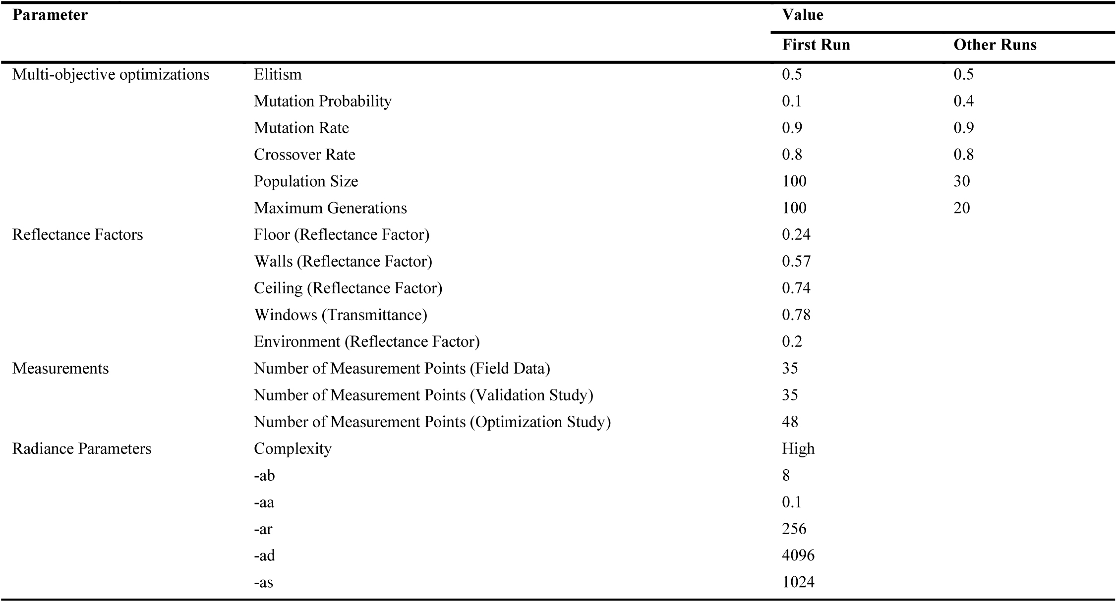
Table 1. Summary of Literature review.
2.3.3. Multi-objective optimization settings
The values for the parameters of multi-objective optimizations vary based on the aim of different studies. Table 1 shows the values that were used in this study. The first row was used according to a previous study [19] but the simulation was terminated after the 54th generation since no new significant results had been added to the simulations results. Accordingly, this study proceeded with a reduced maximum number of generations based on the simulation parameters of two other studies in engineering that showed 20 generations are enough for achieving accurate results [38,39]. The simulation variables are defined based on the “Floor Ratio” and “Window Length” in the simulation files. Window Length varies based on the maximum available length (0.1 – 4 m) with 0.1 m increments. The Floor Ratio also varies from 1 to 100% with 1% increments.
2.3.4. Radiance parameters
In this study, high complexity was used for calculations. The main parameters that may affect the results are set as follows; Ambient Accuracy (-ab) = 8, Ambient Accuracy (-aa) = 0.1, Ambient Resolution (-ar) = 256, Ambient Divisions (-ad) = 4096, Ambient Super-samples (-as) = 1024. High complexity in HoneybeePlus sets the other Radiance parameters for calculations. The error in this method is below 20% [24].
2.4. Dynamic metrics for multi-objective optimization
Metrics for measuring the daylight-related issues based on the climate of a region are known as dynamic metrics. Using this approach is called Climate-based Daylight Modeling (CBDM) which has three important metrics, including Daylight Autonomy (DA), Useful Daylight Illuminance (UDI-a), and Annual Sunlight Exposure (ASE1000,250). Accordingly, these metrics were used in this study and are defined in this section.
Daylight Autonomy (DA): is defined as the percentage of the number of hours that a particular daylight level in buildings is exceeded in a given year [22]. On the other hand, sDA is defined as the percentage of floor area that receives at least 300 lux for at least 50% of the annual occupied hours [21]. DA was chosen in this study because it shows the exact percentage of the number of hours that a particular daylight level is met (exceeded). This can be used in the future for studies on blinds, shades, etc. This metric is maximized in this study and the x-axis (dark red) in graphs represents this metric (Figs. 3 and 4).
Figure 3
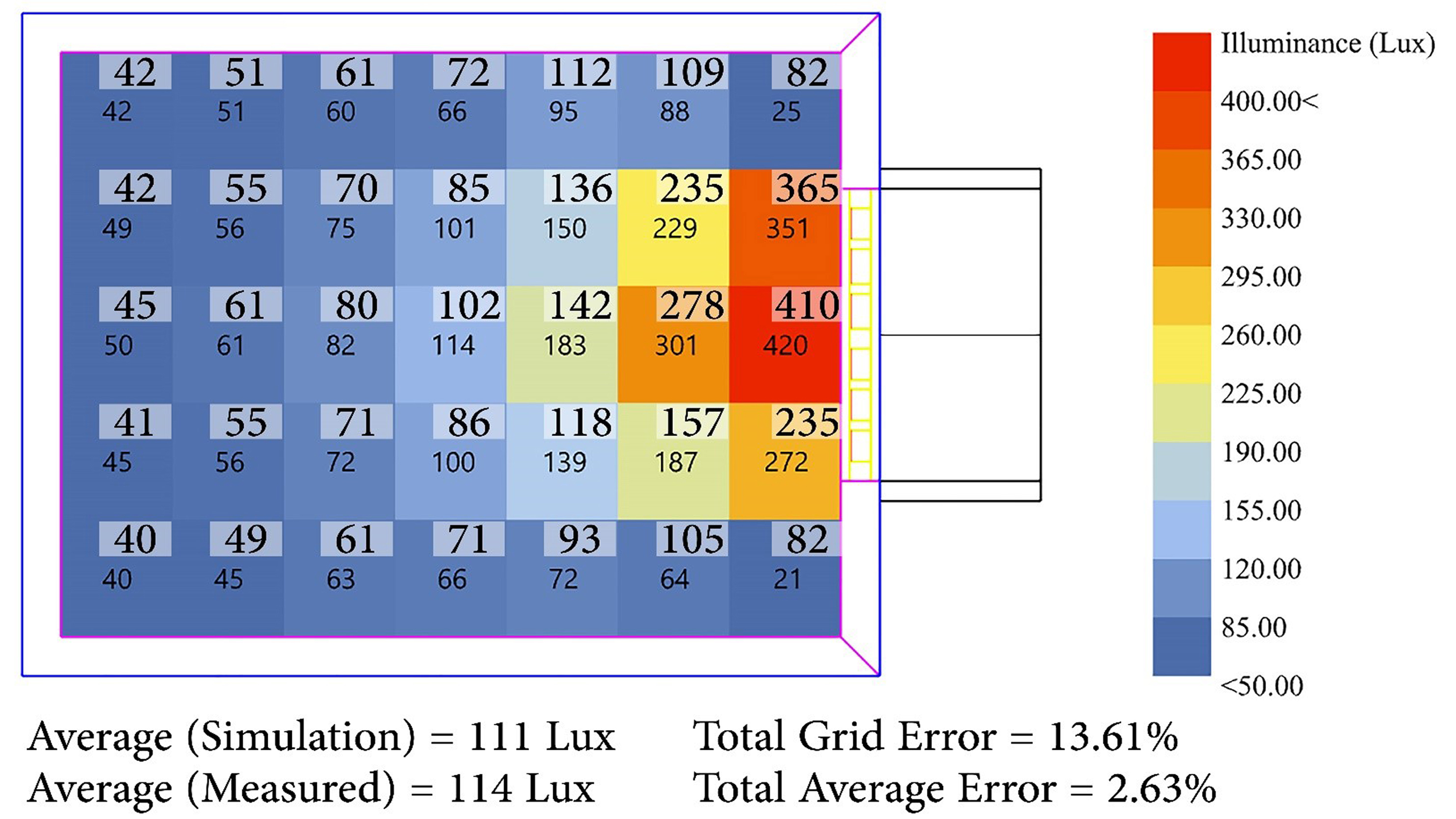
Fig. 3. Model validation against field measurements.
Figure 4
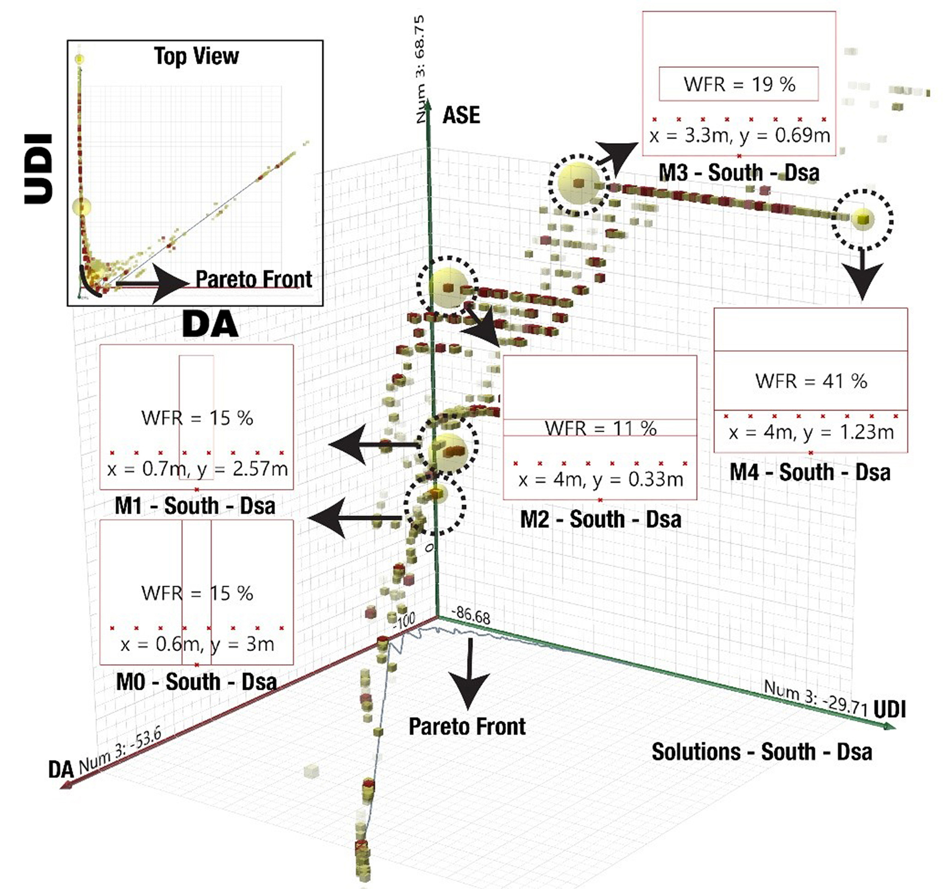
Fig. 4. The analyses results for the southern facades of the Dsa climate.
Useful Daylight Illuminance (UDI-a): is a dynamic metric that is defined as the percentage of the occupied time that a target range of illuminances at a measuring point in space is met by daylight. Daylight illuminance between 300 and 3000 lux is considered desirable. Rooms with illuminance levels below 300 lux may need artificial lighting in the range of 100 to 300 lux are considered effective either as the sole source of illumination or in conjunction with artificial lighting [20]. This metric is maximized in this study and the y-axis (light green) represents this metric (Fig. 4). Coupling DA with UDI-a helps the designers to determine the effect of possible glare for illuminance levels of about 3000 lux as well as illuminance levels below 300 lux.
Annual Sunlight Exposure (ASE1000,250): is a metric for measuring the amount of space that receives too much direct sunlight which may result in increased cooling loads or visual discomfort (glare). The metric is defined as the percentage of floor area that receives at least 1000 lux (direct sunlight) for at least 250 occupied hours per year [21]. This metric is minimized in this study and the z-axis (dark green) represents this metric (Fig. 4).
Furthermore, Occupancy schedules are of significant importance to new dynamic metrics of daylighting such as Useful Daylight Illuminance (UDI-a) [40]. Dynamic metrics of daylight calculations, such as Annual Sunlight Exposure (ASE1000,250) or Daylight Autonomy (DA), also depend on weather conditions [41]. In this study, the general 8 AM to 5 PM occupancy schedule is used. This is an hour less than the standard schedule of 8 AM to 5 PM since it has been modified to match the local working hours.
2.5. HypE algorithm and pareto approach
Multi-objective optimization in this study was based on the HypE algorithm which is an improved version of the NSGA-II algorithm [29,30]. This study used Octopus version 0.4 as an interface for carrying out the study [28]. The results are picked based on the Pareto approach [42]. In this approach, picking the best solution based on simulation results in a multi-objective optimization differs from single-objective optimizations. In this approach, for instance, solution A dominates other solutions if solution A outperforms or performs as efficiently as other solutions in at least one objective. On the other hand, solutions do not dominate each other if each specific solution outperforms the other in different objectives. A graphical front, known as Pareto front, is created when the results are available.
In this study y- and x-axes are UDI-a and DA that should be maximized while the z-axis is ASE1000,250 which should be minimized. Objectives are minimized by default in multi-objective optimization studies in Octopus. This means that mathematically, any given positive parameter is minimized. Mathematically, these parameters that should be maximized are multiplied by -1 so that they are maximized in optimizations. Therefore, the objective should be multiplied by -1 for maximization. Hence, UDI-a and DA are represented by negative numbers. It is just a mathematical equation for maximizing the objective. As a result, the best solution would be the closest solution to the origin of the three-dimensional cartesian graph. For clarity, the axes for UDI, DA, and ASE1000,250 are marked on all figures.
2.5.1. Best solution criteria
For picking up the best solution, Octopus as the optimization engine provides a user-friendly interface that allows researchers to evaluate each solution elaborately. Although this cannot be shown on the figures since they lack the interactivity of the interface, the files with the Octopus interface can be provided upon request. In this study, the closest most optimum solution is defined as M0 which stands for Model 0. Similarly, M1 represents the optimum solution with increased ASE. This decision was made since ASE1000,250 can be controlled using occupant behaviors such as closing curtains. M2, M3, and M4, which have a higher value for UDI, represent the author’s evaluation of other solutions in the Octopus interface. These solutions were picked for evaluation of the size of windows. Subsequently, a suggested minimum standard is suggested by using the optimum solutions (M0 and M1), and these evaluated solutions (M2, M3, and M4) in Octopus. The main selection criterion for the percentages of WFRs is a height of 60 cm so that occupants can have a view of the outside. Through these criteria, this article investigates the optimum solutions and suggest minimum required WFRs along with the Proportion Range (PR) for each cardinal direction in the two Csa and Dsa climates. The PR value is introduced since a specific WFR can be achieved by different lengths and heights. The PR suggests the best proportion for achieving a specific PR.
3. Results and discussion
3.1. Validation
The field data and simulated illuminance levels are shown in Fig. 3. The numbers with white background represent the in-situ measurements while the others are from the simulation. The error for average illuminance levels was below 3% while point-by-point analyses show an error below 15%. This is in accordance with previous validation studies that indicated the error in Radiance is below 20% which is acceptable in simulations [24,37,43]. It should be noted that metrics used in this article all rely on the average illuminance level which has an error below 3%.
3.2. Multi-objective optimization of southern facades
Figures 4 and show the analyses results for the southern facades of the Dsa and Csa climates. As described in the research method, the best solution is the closest solution to the origin of the three-dimensional Cartesian coordinate system. Accordingly, model number 0 (M0) is the best solution for both climes. M1 in the Dsa climate (Fig. 4) is the next appropriate solution. Solutions from M0 to M1 can be considered as the best solutions. However, M0 is the best solution based on Daylight Autonomy (DA), Useful Daylight Illuminance (UDI-a), and Annual Sunlight Exposure (ASE1000,250). M2 in Fig. 4 and M1 in Fig. 5 are marked as the solutions with maximum DA and UDI-a but with an increased ASE. These solutions were investigated to evaluate the effect of ASE1000,250 on the optimum WFR. It is observed that an elevated ASE1000,250 is associated with the horizontal orientation of windows in both climates but it is not necessarily associated with the WFR percentage.
Figure 5
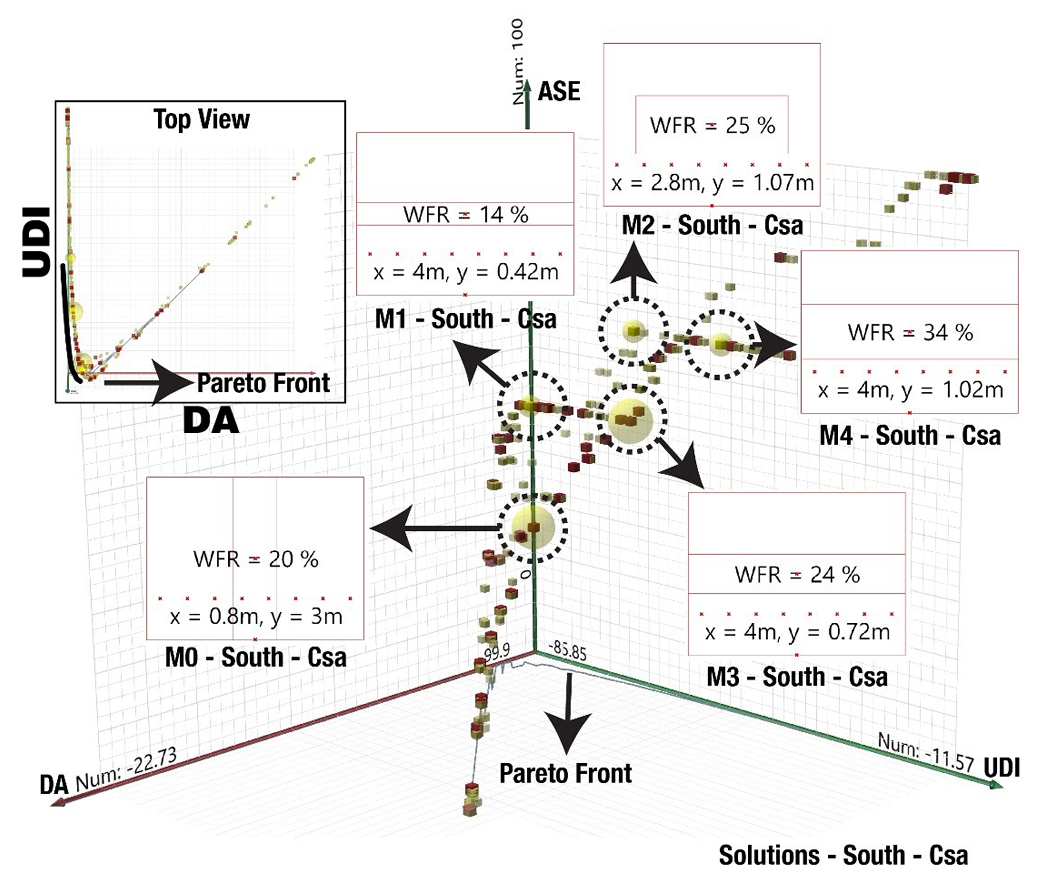
Fig. 5. The analyses results for the southern facades of the Csa climate.
Table 2 shows the analysis results for the southern facades. Furthermore, in the tables, X and Y labels on the facades (figures) represent the length and height of the windows while X and Y values in the table represent the values that can create these specific windows. According to this table, M0 represents the best solution for achieving the maximum DA and UDI-a and the minimum ASE1000,250 in both climates. It is observed that a horizontal orientation for windows increases the ASE1000,250 significantly. For instance, M1 in the Dsa climate has an area of 15% while the same model in the Csa climate has an area of 14% but the ASE1000,250 increased from 27% to 50% due to the difference in orientation of the two selected solutions (M1 in the Dsa and Csa).
Table 2
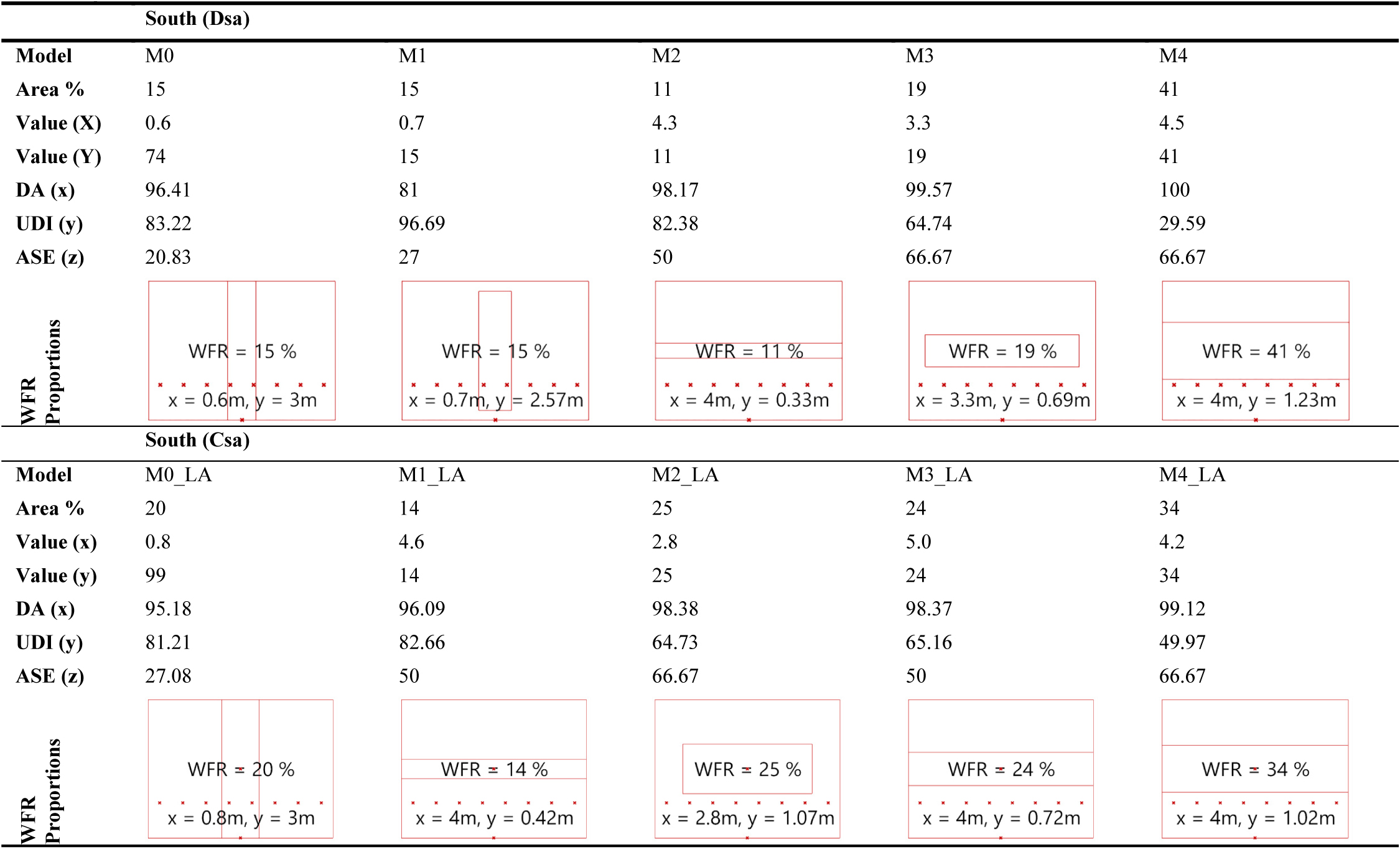
Table 2. Optimization results for the southern facades.
While the best solutions in the Dsa and Csa climates may be visually appealing to occupants, the preference goes to M3 in the Dsa climate and M2 in the Csa climate based on the standards for the minimum height of windows in residential buildings. However, the accepted local standards may be different for other types of buildings such as offices. Another major observation is in the analyses of the values of DA and UDI. While increasing the WFR increases the DA, it decreases the UDI. This means that illuminance levels surpass the 3000 lux threshold by increasing the WFR and as a result, the UDI-a decreases.
3.3. Multi-objective optimization of northern facades
Figures 6 and 7 show the results for the northern facades. In the Dsa climate, the ASE1000,250 values vary but its values are zero in the Csa climate. These results may be due to the location of the test models in the Dsa and Csa climates. The test model for the Dsa is located at 35.3219° N and 46.9862° E while the test model for the Csa is located at 34.0522° N, 118.2437° W. The difference in the values of ASE1000,250 is a direct result of sun position in these two different locations since one is closer to the equator and the other is farther. It is unlikely that climatic conditions such as the number of cloudy days create this particular issue since the ASE1000,250 values are also low in the Csa climate (Table 3).
Figure 6
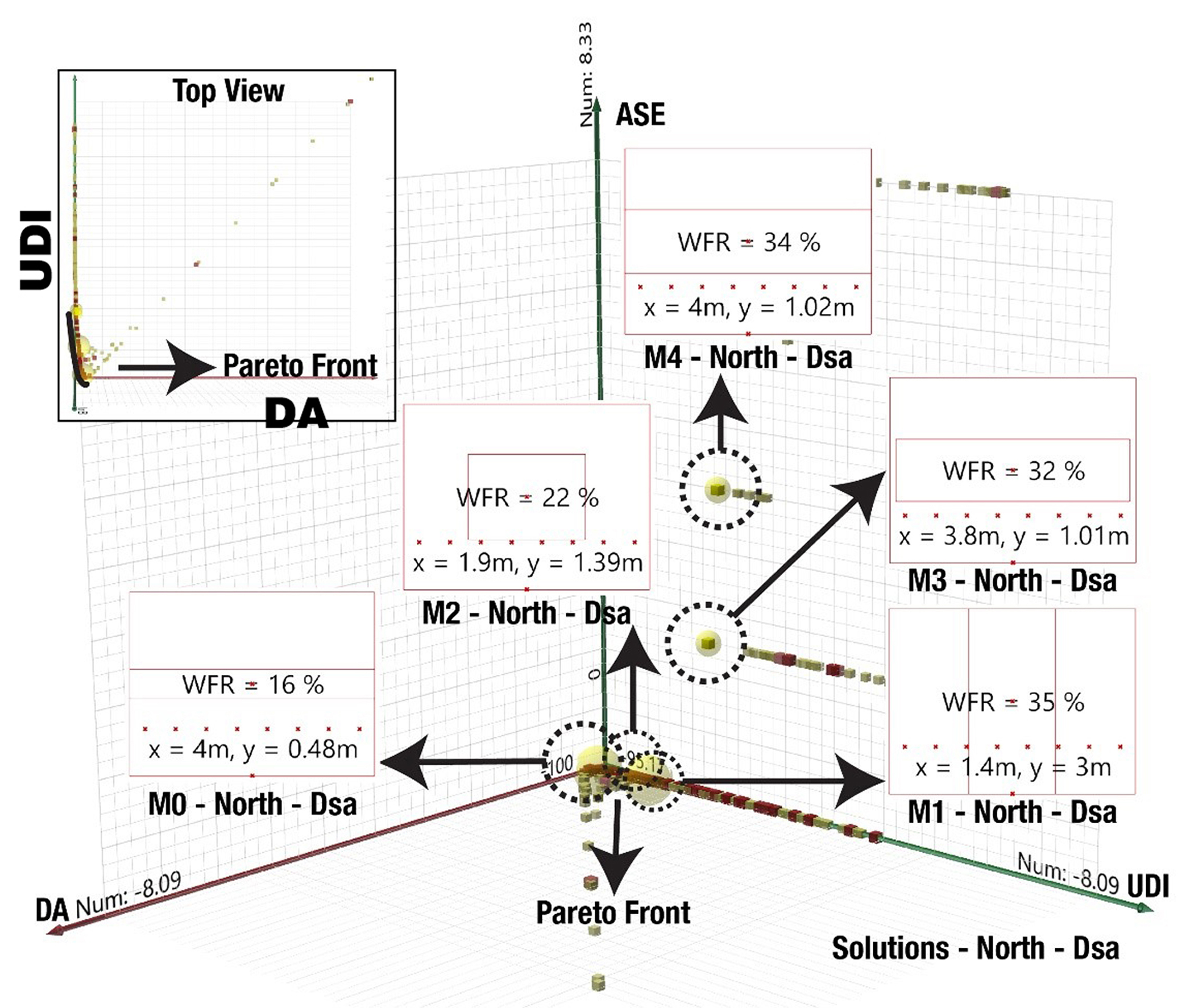
Fig. 6. The analyses results for the northern facades of the Dsa climate.
Figure 7
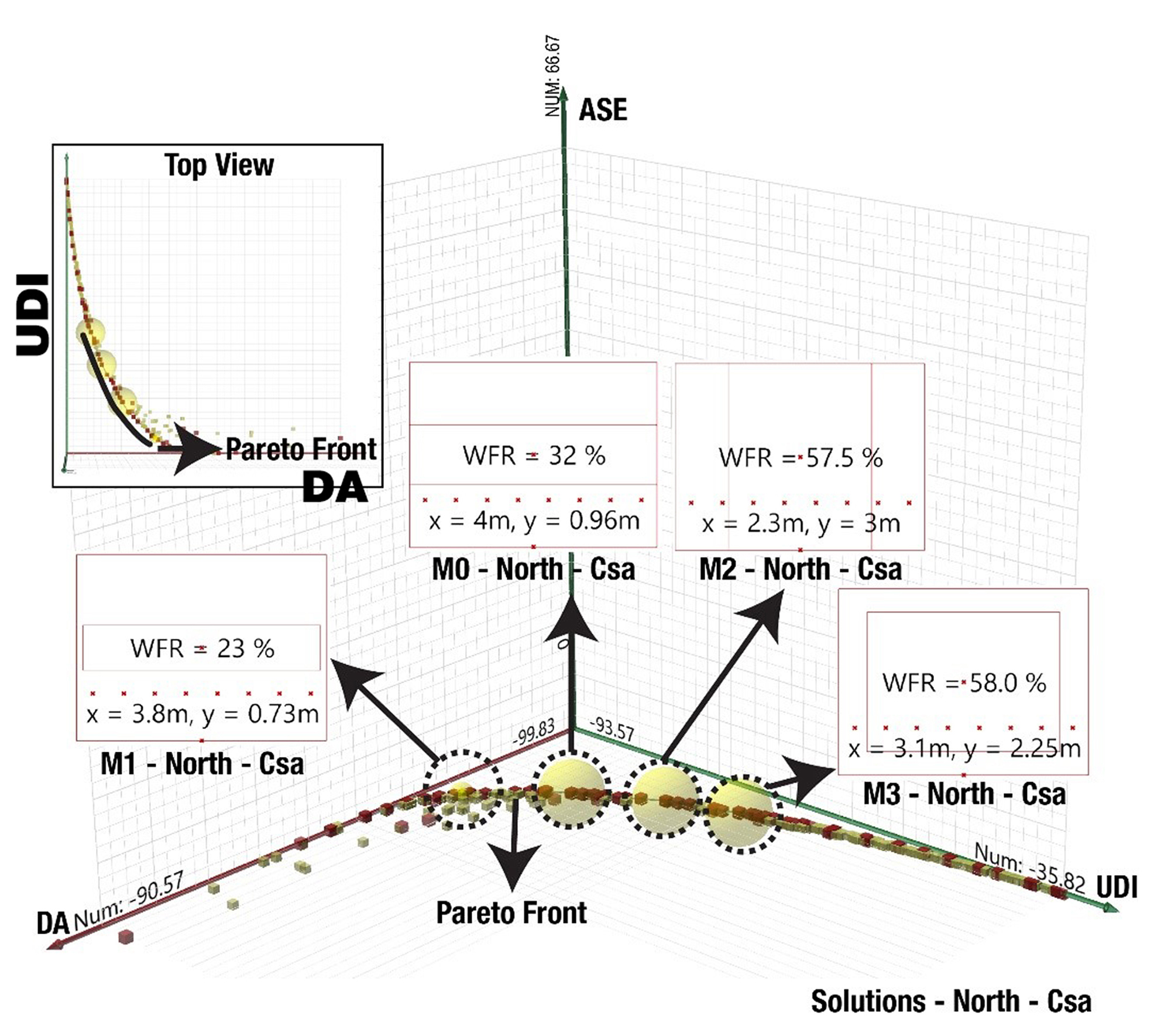
Fig. 7. The analyses results for the northern facades of the Csa climate.
Table 3
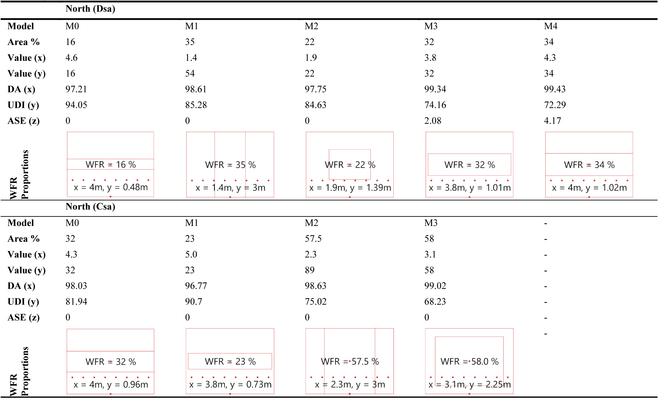
Table 3. Optimization results for the northern facades.
The results show that the best solution for the Dsa climate is a 16% WFR although the height of the window may not be visually appealing in this scenario. Since there is little to no ASE1000,250 involved in the northern façade for the Dsa climate, both M1 and M2 solutions might be better options for a view of the outside (Table 3). However, M3 and M4 may surpass the 3000 UDI-a threshold since its percentage is below 75%.
On the other hand, the best solution for the Csa climate in Fig. 7 shows that the height of the window is visually appealing in comparison to the other solutions. Although it is chosen as the best solution based on its proximity to the origin of the graph, its UDI-a is slightly lower than solution M1 (Table 3).
3.4. Multi-objective optimizations of eastern facades
Figures 8 and 9 show the results for the eastern facades. The eastern façade, similar to the western façade, receive sunlight partially during the day. As a result, the ASE1000,250 metric becomes critical here since the optimization should look for the best solution that is applicable in the presence and absence of direct sunlight. As a result, solution M0, as the best solution, as well as solutions M1 and M2 may not be visually appealing in the Dsa climate. Similarly, in the Csa climate, M0, as the best solution, and M1, as the second-best solution, may not be visually satisfactory for residential buildings since they are providing a little view of the outside.
Figure 8
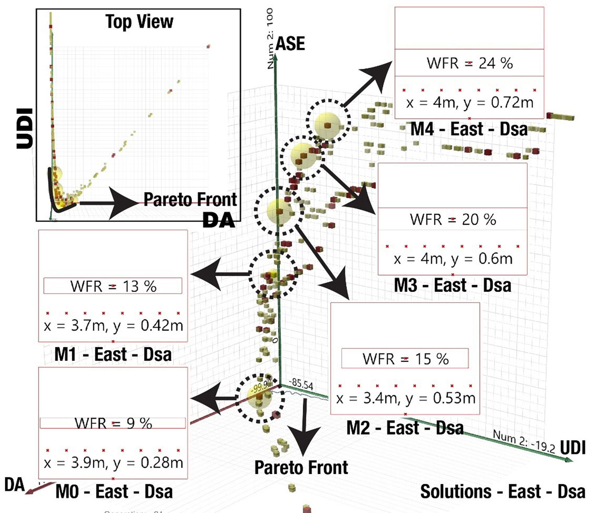
Fig. 8. The analyses results for the eastern facades of the Dsa climate.
Figure 9
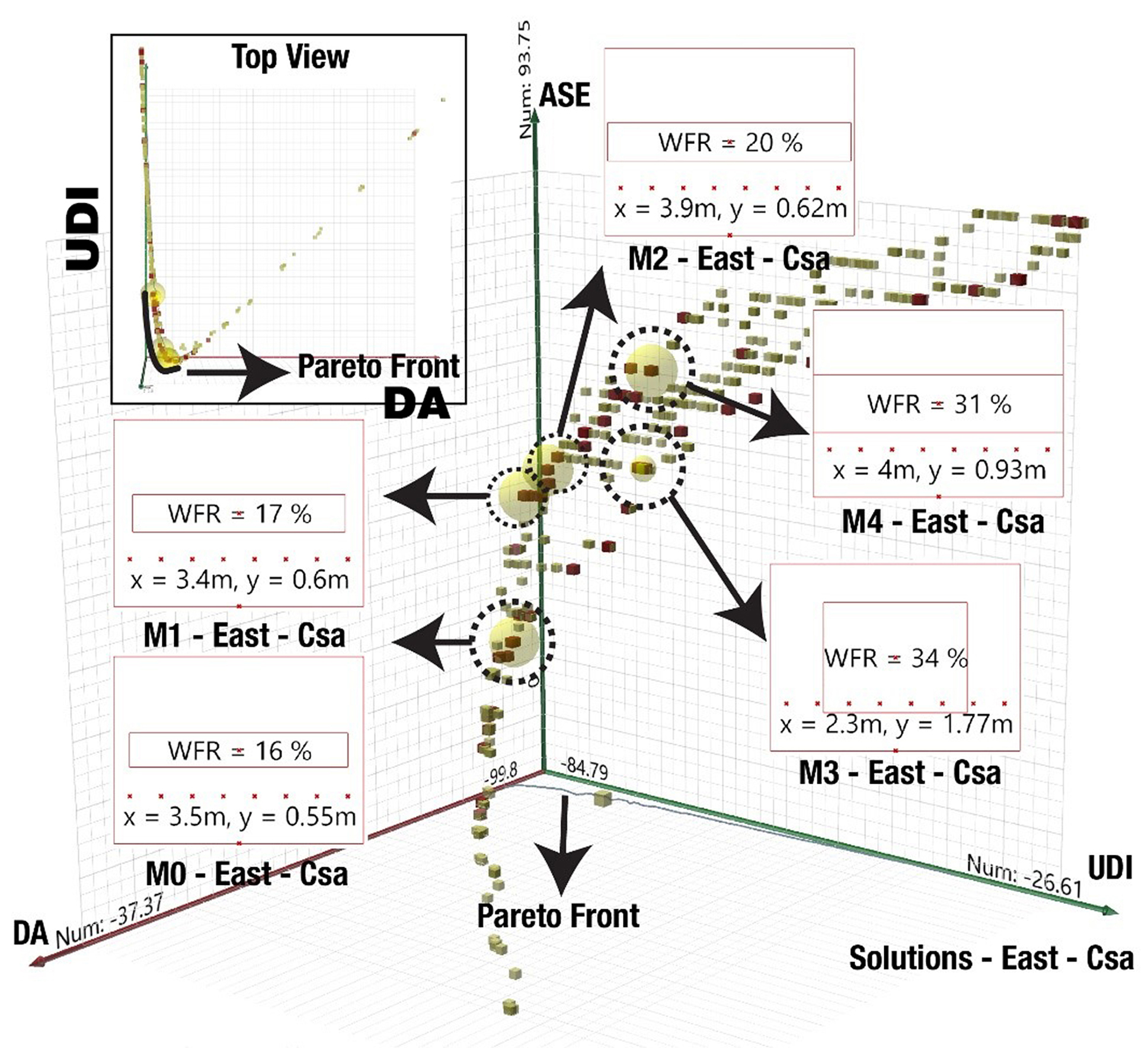
Fig. 9. The analyses results for the eastern facades of the Csa climate.
In contrast, solution M3 in the Dsa climate and M2 in the Csa climate are better options visually but they have significantly higher ASEs that may result in further problems in the building (Table 4). M0 in the Dsa climate and M0 in the Csa climate with ASEs of 0 and 22.92% are the best solutions according to the results of optimization. There is an interesting observation in the Csa climate between M3 and M4. While M4 has a lower WFR, it resulted in a higher ASE1000,250 which is not desirable. This issue is discussed in section 4.1.
Table 4
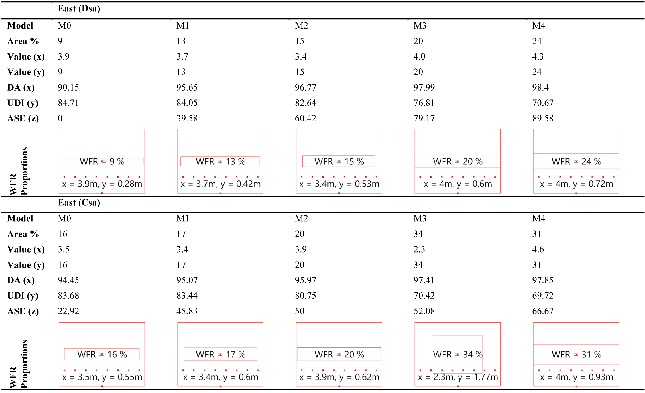
Table 4. Optimization results for the northern facades.
3.5. Multi-objective optimizations of western facades
Figures 10 and 11 show the results of analyses for the western facades in the Dsa and Csa climates. Similar to the eastern facades in the Dsa climate, M0 is the best solution based on optimization results but its proportions may not be as appealing as M2 or M3. In contrast, M1 in the Csa climate is the best optimization solution and provides a sufficient proportion of outside views.
Figure 10
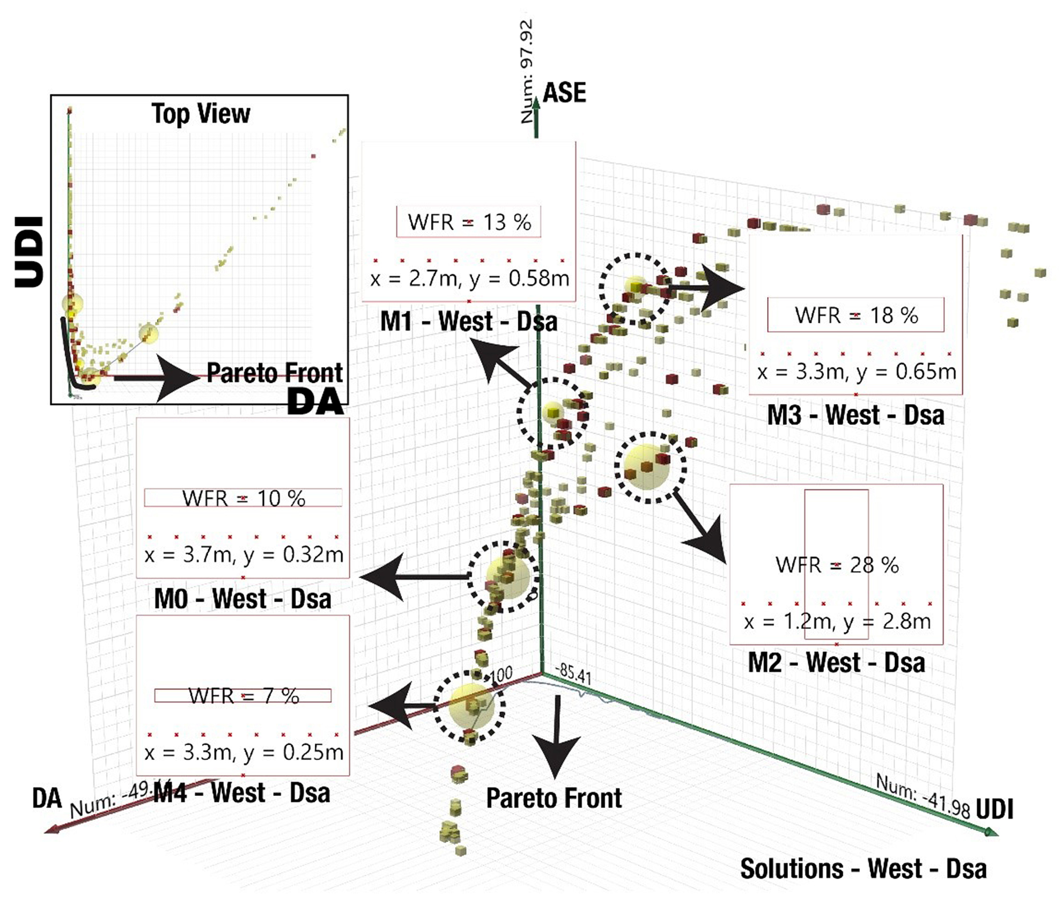
Fig. 10. The analyses results for the western facades of the Dsa climate.
Figure 11
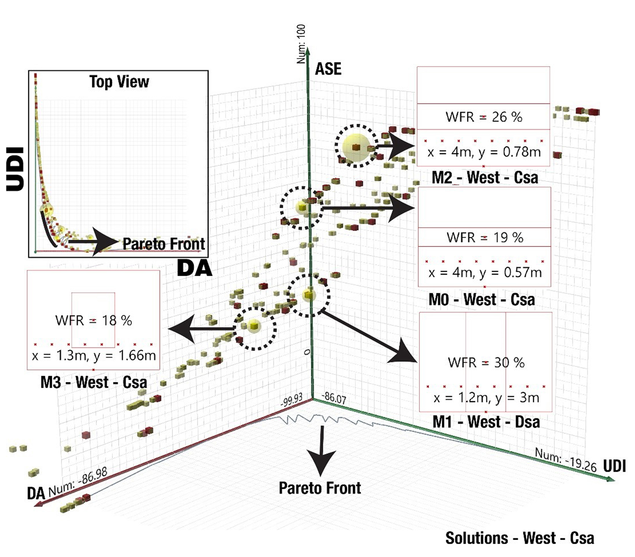
Fig. 11. The analyses results for the western facades of the Csa climate.
While optimization could achieve significantly low ASEs in southern, eastern, and northern facades, finding a solution with a low ASE1000,250 was not possible in the Csa climate based on the results in Table 5. The best solution is M1 with an ASE1000,250 of 39.58% while ASEs around 20% were observed in other directions in both climates. The significant difference between the metrics in the Dsa and Csa climates is because of the sun position in their geographical positions and climatic conditions such as the number of cloudy days.
Table 5
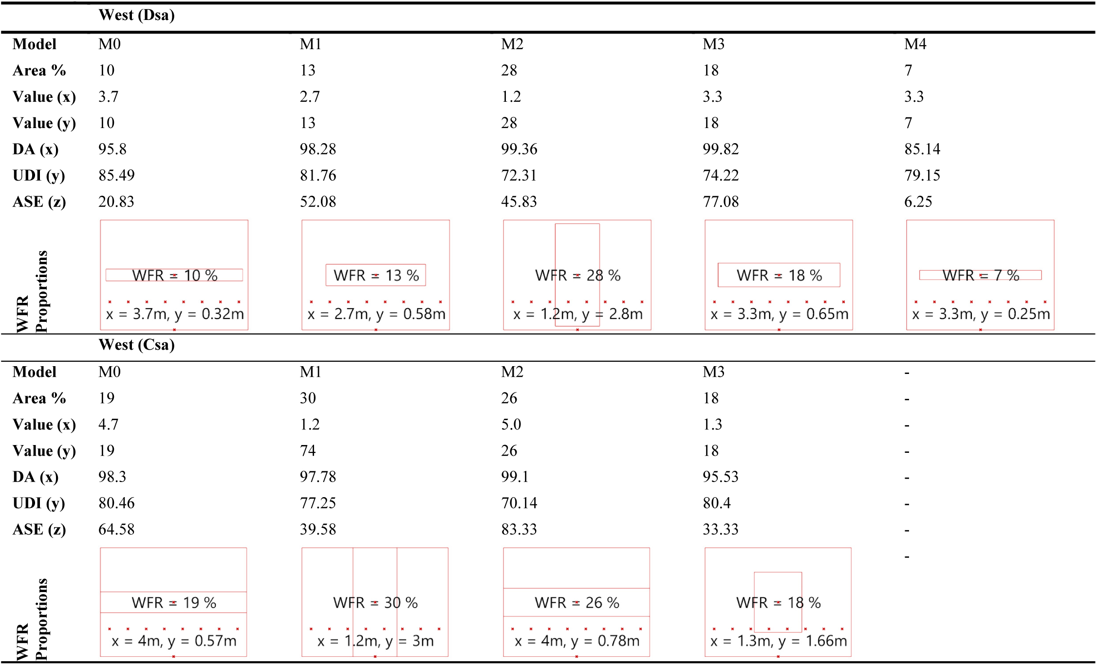
Table 5. Optimization results for the northern facades.
4. Discussion
To avoid the complexity of interpretation, the optimum proportions were not discussed in the previous section. At the end of this section, the best solutions of optimum window sizes as well as visually appealing solutions with a height of at least 60 cm are presented. Also, the worst condition on the Pareto front is discussed. But before suggesting the aforementioned window sizes based on the WFR, three issues should be discussed including the shape and orientation of windows, the relationship between the work plane at the height of 76 cm and the position of windows, and the effect of measurement points on the outcome.
4.1. Shape and orientation of windows
As the results of this paper suggest, east-, north-, and west-facing windows of buildings in the Dsa climate and east- and north-facing windows in the Csa climate benefit from the horizontal orientation of windows (vertical/horizontal positions based on its longest edge) based on the optimization results. Vertical windows may be deemed optimized due to the ASE1000,250 metric in other directions. The results show horizontal windows increase the ASE1000,250 value in simulations. Therefore, it would be better to provide suggestions for implementation in the Dsa and Csa environments based on horizontal orientation and avoid excessive sunlight through preventive measures such as behavioral actions of closing and opening curtains or using shading devices.
Comparing the results of the present study with previous studies on windows orientation can confirm the findings of this study. A previous study showed that horizontal windows result in higher illuminance levels in the side axes (2% higher) while its performance in the central axis is poorer than the square windows [44]. The results of the present study do not confirm any benefit associated with square windows. Similarly, another study showed that office employees prefer window-walls as their first preference and the horizontal windows as their second while the square windows and other shapes were their fourth and last preferences, respectively [45]. In addition to occupants’ behavioral preference, a study on window design in architecture showed horizontal windows produce higher energy-saving than any other type in the northern facades in London, the UK [46]. In a study on the west- and east-facing rooms, continuous horizontal windows performed better than other types of windows and separate windows with the same glazing ratio in a temperate-dry climate [47]. Similar studies show the benefit of windows that are stretched horizontally [48]. Horizontal windows are also considered effective in improving circadian rhythms [8].
As a result, it can be concluded that the benefits of horizontal windows outweigh the vertical windows that were suggested as the most optimized shape based on the ASE1000,250 metric. As a result, suggestions for future use based on the WFR are better to be designed horizontally.
4.2. Work plane and the position of windows
The work plane is essentially what the metrics work based on since it is the measurement plane as well. However, the percentage of windows that are below the height of 76 cm (The distance of work plane from the ground) does not have a direct effect on the outcome of results but they have a secondary effect since the daylight is not being radiated on the work plane directly. The secondary effect is the reflection of light from the surfaces. This is the secondary effect that is capable of increasing the overall illuminance of rooms through reflection.
In contrast, the distance of windows from the plane or sill height can play a significant role in predictions. For instance, a window that has a sill height of 0.76 helps the work plane to receive daylight from its starting edge while a window that is placed above the work plane, a sill height of 1.2 for instance, can provide better daylight for the farther edge of the work plane. These complexities require local simulation for every different design. As a result, as described earlier in the research method section, this study used a basic model of 12 m2 that can be expanded for each space. This enables us to introduce a new ratio for windows in different climates. This study defines the “Proportion Ratio” (PR) as the ratio of the horizontal edge of windows to the vertical edge. This ratio helps designers to design windows efficiently for receiving maximum daylight and avoid adverse effects such as glare. The values for this ratio in the Dsa and Csa climates are offered in Section 4.4.
4.3. Achieving the optimum window sizes for the dsa and csa climates
In this section, the optimized optimum window sizes as well as suggestions for broader application in the Dsa and Csa climates are presented. Table 6 shows the WFRs based on the results of simulations for the four cardinal directions in both climates. The main selection criterion for the percentages of WFRs is a height of 60 cm so that occupants can have a view of the outside. Although such a principle is not actively pursued in many design circumstances since designers may want to limit the interaction with outside, this paper assumes a minimum of view for occupants because this paper assumed a 12 m2 space, a base model for main living areas, as the main module for designers and future studies on daylighting. Accordingly, the minimum suggested WFR for the Dsa and Csa are presented in Table 1. In this table, the “Most Optimized Solution” is the most optimized solution without any further processing such as evaluation for the portion of outside views for occupants. The “Suggested Standards” are solutions that have been further processed to meet a minimum for the portion of outside views. The use of PR is also demonstrated in this table. The “PR Orientation” represents the proportion of the window while “PR Value” represents the proportion of the height of the window divided by its length. This value is suggested to be between 0.1 and 0.5 (0.1 ≤ PR ≤ 0.5) based on the façade of the windows. The least PR value is for west-facing windows since these windows do not provide visually appealing daylight. As a result, designers try to avoid using large proportions in the northern hemisphere. Although the WFR for the south-, east-, and west-facing windows is 20%, the minimum sill height is different for them since it affects the dynamic metrics as discussed in Section 4.3. Similarly, the sill height of north-facing windows in the Dsa climate is equivalent to the height of the work plane (76 cm). This table helps designers to have minimums for a base module during their early design stages. The importance of this table is in its ability to provide designers minimum requirements for each space for sufficient daylighting as well as visual comfort. During the early stages of design, architects and designers can achieve optimized indoor environments in terms of daylight and visual comfort. These numbers then can be used further for indoor environmental quality (IEQ) assessments. Moreover, this table can help to avoid overheating and underheating which are unfortunately neglected in modern luxurious designs in these two climates. The trend of maximizing the outdoor views imposes significant energy demand on buildings that can now be avoided by using the following table. The table presents the minimum required WFRs in buildings for efficient daylighting.
Table 6
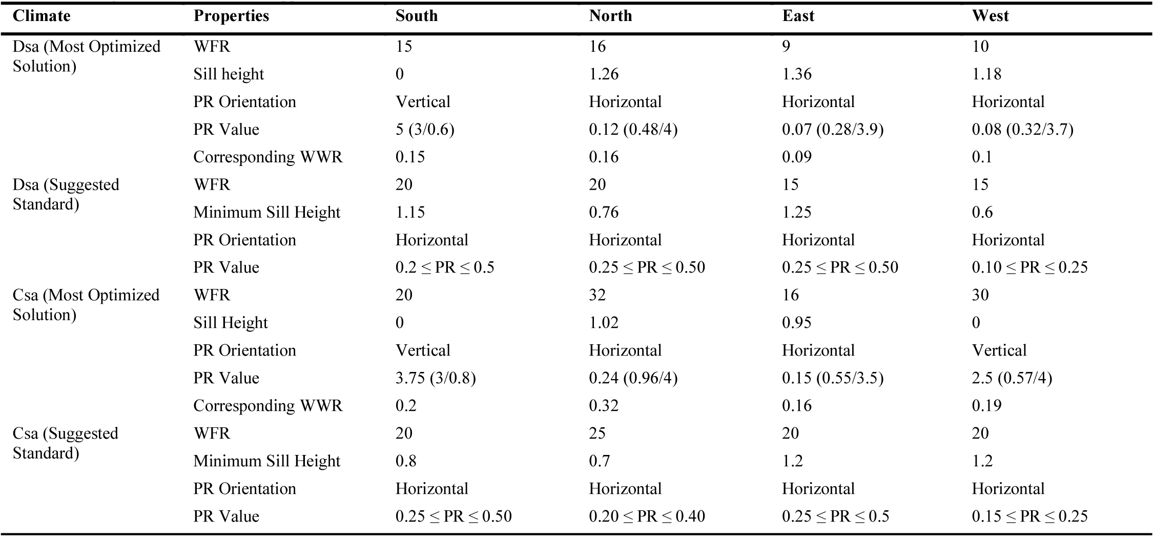
Table 6. Optimization results for the northern facades.
In Table 6, the corresponding WWR is defined for the optimum solution for comparison since they had an exact PR value. Similar to a previous, the northern façade requires a higher WFR [49] although the overall WWR values are lower in this study. This is due to some fundamental differences. The model in the cited article is 2.4 m x 4.2 m which shows the depth of penetration plays a significant role in determining the WWR which is the same as another study that considered various depths [50]. In this regard, the WFR is more useful since the effect of light shelves and other measures can improve the depth of penetration of light in the building. Another limitation with the cited article is that it sets -ab parameter in Radiance to 5 which recent studies showed that it might not be accurate enough [37]. For the Csa climate, the WWR values are almost in accordance with a previous study on the Csa climate [51]. A review article on potential energy savings of WWRs above 30% concludes that increasing the WWR above does not improve the energy use and lighting [52]. In the present study, the minimum required WFR suggests the same thing as they are driven from the optimum solution for daylighting. Another article also suggests that the minimum WWR is normally 20% based on studies in 3 cities in Germany (Berlin) and Italy (Turin and Catania) [53]. Overall, it can be observed that the minimum suggested as well as the optimum solutions in Table 6 are close to the minimums in the aforementioned studies. As a result, the suggest WFR can play be set as the minimum required WFRs in buildings codes while they simultaneously suggest opportunities for future studies to investigate the depth of penetration of light, uniformity of daylight distribution, and the effect of light shelves, etc. for efficient daylighting and optimum sizes of windows.
Conclusion
This paper investigated the minimum size of windows for efficient daylighting through multi-objective optimization in the Csa and Dsa climates since there has been no study or standard on the minimum size of windows based on the WFR and climate classification. Three dynamic metrics of CBDM, including UDI, DA, and ASE, were used for conducting the multi-objective optimization. The results were extracted and interpreted based on the Pareto front approach.
The results showed the most optimum solutions for windows. To create a robust minimum standard, the range of solutions were explored and solutions for WFRs with a minimum height of 60 cm for windows were picked to provide a sufficient view of the outside. In addition, this study showed the minimum sill height is of significant importance. As a result, this study introduces the minimum sill heights for creating a minimum standardized WFR. Furthermore, the PR as a new indicator (independent variable from daylight) for efficient daylighting was introduced that sets the minimum ratio for the orientation of windows (horizontal/vertical). These findings can be used worldwide in the Csa and Dsa climates. This study is the first study that suggests minimums based on the WFR and introduces a ratio and standard sill heights for the windows in addition to the percentages of WFR. The results of this study can help the legislative body to adjust their minimum requirements based on these findings. Building codes are normally considering minimums for designing buildings. As a result, the upper limit of the window sizes is rarely suggested in building codes. This is the main reason that nowadays more and more curtain walls and 100% WFR is being used in residential and commercial developments. Therefore, legislative bodies can use this study to create a foundation for maximizing the efficiency of an envelope in terms of daylight and visual comfort by an optimum WFR and PR value range that has the potential to prevent overheating or underheating of buildings. Although energy efficiency was not considered in this study directly, it can be used in future studies based on these numbers and evaluations of the PR value range. However, the ASE1000,250 as an indicator for potential glare and solar heat gains suggests that these numbers can optimize the envelope.
There are some issues to consider for future studies. This study considers the WFR based on the center point of surfaces. For instance, if a design situation imposes the use of side windows, efficient daylighting requires modeling. In such scenarios, a vertical window may work more efficiently. Moreover, sun position in the cities that were selected for the Csa and Dsa climates may differ from the location of projects in the future but it can be concluded that cities on the same circle of latitudes can use the suggested WFRs without any further considerations. Moreover, some limitations are associated with this study: 1) The uniformity ratio was not considered in this study. The uniformity ratio creates a better environment for visual comfort and is a major part of indoor environment quality studies 2) impact of windows on energy demand was not considered in this study since EnergyPlus and Radiance use different methods of calculations. Another major limitation is that this study did not consider a range of visible transmittance for windows. This is an important issue that can be studied in the future based on different manufacturers. Other limitations associated with this paper are the occupants’ assessment of the location of windows as well as the aesthetics. This study is the first try to create a global database for efficient daylighting based on climate classifications and the WFR. It is recommended that future studies try to document the optimum WFRs for other climate classifications and different cities.
Declaration of competing interest
The authors report no conflicts of interest.
References
- Z. Li, H. Chen, B. Lin, Y. Zhu, Fast bidirectional building performance optimization at the early design stage, in: Building Simulation, 2018, pp. 647–661, Springer. https://doi.org/10.1007/s12273-018-0432-1
- T.M. Echenagucia, A. Capozzoli, Y. Cascone, M. Sassone, The early design stage of a building envelope: Multi-objective search through heating, cooling and lighting energy performance analysis, Applied Energy 154 (2015) 577–591. https://doi.org/10.1016/j.apenergy.2015.04.090
- Y. Zhai, Y. Wang, Y. Huang, X. Meng, A multi-objective optimization methodology for window design considering energy consumption, thermal environment and visual performance, Renewable Energy 134 (2019) 1190–1199. https://doi.org/10.1016/j.renene.2018.09.024
- K. Alhagla, A. Mansour, R. Elbassuoni, Optimizing windows for enhancing daylighting performance and energy saving, Alexandria Engineering Journal 58 (2019) 283–290. https://doi.org/10.1016/j.aej.2019.01.004
- C.E. Ochoa, M.B.C. Aries, E.J. Van Loenen, J.L.M. Hensen, Considerations on design optimization criteria for windows providing low energy consumption and high visual comfort, Applied Energy 95 (2012) 238–245. https://doi.org/10.1016/j.apenergy.2012.02.042
- T.J. Dabe, V.S. Adane, The impact of building profiles on the performance of daylight and indoor temperatures in low-rise residential building for the hot and dry climatic zones, Building and Environment 140 (2018) 173–183. https://doi.org/10.1016/j.buildenv.2018.05.038
- M.L. Amundadottir, S. Rockcastle, M. Sarey Khanie, M. Andersen, A human-centric approach to assess daylight in buildings for non-visual health potential, visual interest and gaze behavior, Building and Environment 113 (2017) 5–21. https://doi.org/10.1016/j.buildenv.2016.09.033
- I. Acosta, M.Á. Campano, R. Leslie, L. Radetsky, Daylighting design for healthy environments: Analysis of educational spaces for optimal circadian stimulus, Solar Energy 193 (2019) 584–596. https://doi.org/10.1016/j.solener.2019.10.004
- J. Mardaljevic, Examples of climate-based daylight modelling, in: CIBSE National Conference, 2006, pp. 1–11, UK.
- Z. Zhou, C. Wang, X. Sun, F. Gao, W. Feng, G. Zillante, Heating energy saving potential from building envelope design and operation optimization in residential buildings: A case study in northern China, Journal of Cleaner Production 174 (2018) 413–423. https://doi.org/10.1016/j.jclepro.2017.10.237
- H.J. Kwon, S.H. Yeon, K.H. Lee, K.H. Lee, Evaluation of building energy saving through the development of venetian blinds’ optimal control algorithm according to the orientation and window-to-wall Ratio, International Journal of Thermophysics 39 (2018) 30. https://doi.org/10.1007/s10765-017-2350-3
- K. Bamdad, M.E. Cholette, L. Guan, J. Bell, Ant colony algorithm for building energy optimisation problems and comparison with benchmark algorithms, Energy and Buildings 154 (2017) 404–414. https://doi.org/10.1016/j.enbuild.2017.08.071
- I. Susorova, M. Tabibzadeh, A. Rahman, H.L. Clack, M. Elnimeiri, The effect of geometry factors on fenestration energy performance and energy savings in office buildings, Energy and Buildings 57 (2013) 6–13. https://doi.org/10.1016/j.enbuild.2012.10.035
- J.-W. Lee, H.-J. Jung, J.-Y. Park, J.B. Lee, Y. Yoon, Optimization of building window system in Asian regions by analyzing solar heat gain and daylighting elements, Renewable Energy 50 (2013) 522–531. https://doi.org/10.1016/j.renene.2012.07.029
- ASHRAE Standard, Standard 901-2019, Energy standard for buildings except low rise residential buildings.
- M. Krarti, P.M. Erickson, T.C. Hillman, A simplified method to estimate energy savings of artificial lighting use from daylighting, Building and Environment 40 (2005) 747–754. https://doi.org/10.1016/j.buildenv.2004.08.007
- J. Gagne, M. Andersen, A generative facade design method based on daylighting performance goals, Journal of Building Performance Simulation 5 (2012) 141–154. https://doi.org/10.1080/19401493.2010.549572
- R.A. Mangkuto, M. Rohmah, A.D. Asri, Design optimisation for window size, orientation, and wall reflectance with regard to various daylight metrics and lighting energy demand: A case study of buildings in the tropics, Applied Energy 164 (2016) 211–219. https://doi.org/10.1016/j.apenergy.2015.11.046
- A. Zhang, R. Bokel, A. van den Dobbelsteen, Y. Sun, Q. Huang, Q. Zhang, Optimization of thermal and daylight performance of school buildings based on a multi-objective genetic algorithm in the cold climate of China, Energy and Buildings 139 (2017) 371–384. https://doi.org/10.1016/j.enbuild.2017.01.048
- J. Mardaljevic, M. Andersen, N. Roy, J. Christoffersen, Daylighting, Artificial Lighting and Non-Visual Effects Study for a Residential Building.
- The Illuminating Engineering Society of North America (IES), LM-83-12: Approved Method: IES Spatial Daylight Autonomy (sDA) and Annual Sunlight Exposure (ASE), Illuminating Engineering Society of North America, New York, 2013. https://doi.org/10.1080/00994480.1990.10747956
- C.F. Reinhart, O. Walkenhorst, Validation of dynamic RADIANCE-based daylight simulations for a test office with external blinds, Energy and Buildings 33 (2001) 683–697. https://doi.org/10.1016/s0378-7788(01)00058-5
- R. Judkoff, D. Wortman, B. O’doherty, J. Burch, Methodology for validating building energy analysis simulations, National Renewable Energy Lab.(NREL), Golden, CO, U.S. https://doi.org/10.2172/928259
- E.S. Lee, D. Geisler-Moroder, G. Ward, Modeling the direct sun component in buildings using matrix algebraic approaches: Methods and validation, Solar Energy 160 (2018) 380–395. https://doi.org/10.1016/j.solener.2017.12.029
- Mostapha Sadeghipour Roudsari, Ladybug Tools, (2020).
- Robert McNeel & Associates, Rhinoceros, (2018).
- D. DiLaura, K.W. Houser, R.G. Misrtrick, R.G. Steffy, The lighting handbook 10th edition: reference and application, Illuminating Engineering Society of North America 120 (2011).
- ETH Zurich, Octopus, (2018).
- F. Peng, K. Tang, Alleviate the hypervolume degeneration problem of NSGA-II, in: International Conference on Neural Information Processing, 2011, pp. 425–434, Springer. https://doi.org/10.1007/978-3-642-24958-7_50
- J. Bader, E. Zitzler, HypE: An algorithm for fast hypervolume-based many-objective optimization, Evolutionary Computation 19 (2011) 45–76. https://doi.org/10.1162/evco_a_00009
- M. Marzouk, M. ElSharkawy, A. Eissa, Optimizing thermal and visual efficiency using parametric configuration of skylights in heritage buildings, Journal of Building Engineering (2020) 101385. https://doi.org/10.1016/j.jobe.2020.101385
- L. Zhang, L. Zhang, Y. Wang, Shape optimization of free-form buildings based on solar radiation gain and space efficiency using a multi-objective genetic algorithm in the severe cold zones of China, Solar Energy 132 (2016) 38–50. https://doi.org/10.1016/j.solener.2016.02.053
- B. Kiss, Z. Szalay, Modular approach to multi-objective environmental optimization of buildings, Automation in Construction 111 (2020) 103044. https://doi.org/10.1016/j.autcon.2019.103044
- E. Neufert, P. Neufert, Architects’ data, John Wiley & Sons.
- Milwaukee Electric Tool Corporation, Instruction Manual, MW700 Standard Portable Lux Meter, Instruction Manual, Milwaukee Electric Tool Corporation (n.d.).
- E. Brembilla, C.J. Hopfe, J. Mardaljevic, Influence of input reflectance values on climate-based daylight metrics using sensitivity analysis, Journal of Building Performance Simulation 11 (2018) 333–349. https://doi.org/10.1080/19401493.2017.1364786
- F. Kharvari, An empirical validation of daylighting tools: Assessing radiance parameters and simulation settings in Ladybug and Honeybee against field measurements, Solar Energy 207 (2020) 1021–1036. https://doi.org/10.1016/j.solener.2020.07.054
- E. Salajegheh, S. Gholizadeh, Optimum design of structures by an improved genetic algorithm using neural networks, Advances in Engineering Software 36 (2005) 757–767. https://doi.org/10.1016/j.advengsoft.2005.03.022
- A. Rezvani, M. Gandomkar, Modeling and control of grid connected intelligent hybrid photovoltaic system using new hybrid fuzzy-neural method, Solar Energy 127 (2016) 1–18. https://doi.org/10.1016/j.solener.2016.01.006
- A. Nabil, J. Mardaljevic, Useful daylight illuminances: A replacement for daylight factors, Energy and Buildings 38 (2006) 905–913. https://doi.org/10.1016/j.enbuild.2006.03.013
- J.L.M. Hensen, R. Lamberts, Building performance simulation for design and operation, Routledge.
- M. Di Somma, B. Yan, N. Bianco, G. Graditi, P.B. Luh, L. Mongibello, V. Naso, Multi-objective design optimization of distributed energy systems through cost and exergy assessments, Applied Energy 204 (2017) 1299–1316. https://doi.org/10.1016/j.apenergy.2017.03.105
- M. Ayoub, 100 Years of daylighting: A chronological review of daylight prediction and calculation methods, Solar Energy 194 (2019) 360–390. https://doi.org/10.1016/j.solener.2019.10.072
- I. Acosta, C. Munoz, M.A. Campano, J. Navarro, Analysis of daylight factors and energy saving allowed by windows under overcast sky conditions, Renewable Energy 77 (2015) 194–207. https://doi.org/10.1016/j.renene.2014.12.017
- I.T. Dogrusoy, M. Tureyen, A field study on determination of preferences for windows in office environments, Building and Environment 42 (2007) 3660–3668. https://doi.org/10.1016/j.buildenv.2006.09.010
- I. Acosta, M.Á. Campano, J.F. Molina, Window design in architecture: Analysis of energy savings for lighting and visual comfort in residential spaces, Applied Energy 168 (2016) 493–506. https://doi.org/10.1016/j.apenergy.2016.02.005
- T. Ashrafian, N. Moazzen, The impact of glazing ratio and window configuration on occupants’ comfort and energy demand: The case study of a school building in Eskisehir, Turkey, Sustainable Cities and Society 47 (2019) 101483. https://doi.org/10.1016/j.scs.2019.101483
- E. Negev, A. Yezioro, M. Polikovsky, A. Kribus, J. Cory, L. Shashua-Bar, A. Golberg, Algae Window for reducing energy consumption of building structures in the Mediterranean city of Tel-Aviv, Israel, Energy and Buildings 204 (2019) 109460. https://doi.org/10.1016/j.enbuild.2019.109460
- M.-C. Dubois, K. Flodberg, Daylight utilisation in perimeter office rooms at high latitudes: Investigation by computer simulation, Lighting Research & Technology 45 (2012) 52–75. https://doi.org/10.1177/1477153511428918
- A. Pellegrino, S. Cammarano, V.R.M. Lo Verso, V. Corrado, Impact of daylighting on total energy use in offices of varying architectural features in Italy: Results from a parametric study, Building and Environment 113 (2017) 151–162. https://doi.org/10.1016/j.buildenv.2016.09.012
- F. Goia, Search for the optimal window-to-wall ratio in office buildings in different European climates and the implications on total energy saving potential, Solar Energy 132 (2016) 467–492. https://doi.org/10.1016/j.solener.2016.03.031
- M.-C. Dubois, Å. Blomsterberg, Energy saving potential and strategies for electric lighting in future North European, low energy office buildings: A literature review, Energy and Buildings 43 (2011) 2572–2582. https://doi.org/10.1016/j.enbuild.2011.07.001
- V.R.M. Lo Verso, G. Mihaylov, A. Pellegrino, F. Pellerey, Estimation of the daylight amount and the energy demand for lighting for the early design stages: Definition of a set of mathematical models, Energy and Buildings 155 (2017) 151–165. https://doi.org/10.1016/j.enbuild.2017.09.014
Copyright © 2020 The Author(s). Published by solarlits.com.

2595
Total views
Citations
SHARE ON


