Citation: Doris A. Chi, An Approach to Determine Specific Targets of Daylighting Metrics and Solar Gains for Different Climatic Regions, Journal of Daylighting 8 (2021) 1-19. https://dx.doi.org/10.15627/jd.2021.1

Figures and tables

Abstract

This study comes from an integrated approach combining daylighting and thermal aspects of building spaces. Several room configurations derived from the combination of four main design variables are tested. Width-to-Depth-Ratio (WDR), Window-to-Wall-Ratio (WWR), orientation, and climate conditions are simultaneously investigated to find the best solutions that enhance the Daylight Availability and, at the same time, diminish solar gains and total energy use (lighting plus cooling and heating). Principal Component Analysis (PCA) is the statistical technique used to outline design guidelines for Mexican climate regions, namely arid, tropical, and temperate. Hence, optimal values for WDR and WWR were recommended for specific orientations and climates. Therefore, PCA is set as the basis of a methodology to define design strategies for specific locations and climates that further lead to updating high-performance standards in buildings at regional levels. Results also showed that climate conditions, such as seasonal cloud cover, temperature, and solar radiation, are crucial when establishing target limits for the actual daylit and over lit areas. The temperate climate was able to endure up to 60% as over lit area. Instead, the arid and tropical climates tolerated up to 50% and 40%, respectively, as over lit areas.

Keywords

Principal components analysis, Daylit area, Over lit area, Total annual energy use

1. Introduction

Daylight has been recognized as a useful strategy in energy-efficient buildings. It can contribute to reducing the use of artificial lighting and active thermal conditioning systems in different architectural buildings [1–3]. However, most daylighting research has taken place in non-residential buildings [4]. Some reviews of the state of the art have shown that both the light and the view through windows contribute to feelings of spaciousness and favourable assessments of room appearance [5]. Other authors have extensively investigated the daylight positive impact on people´s health (effects beyond vision), comfort, and well-being [6–8]. Several lines of research have also shown that increased light exposure by day can promote pleasant mood and feelings of alertness, independent of circadian regulation [7]. On the contrary, lack of access to daylight could be one factor for lower well-being of poor housing quality: An optimal design of healthful housing should include appropriately sized and oriented openings to deliver light and views [4].

Therefore, daylight is an important feature in any building type. The amount of daylight entering a building is mainly through windows. Thus, windows contribute to providing light to the eyes while creating a more attractive and pleasant indoor environment [7]. These openings are also associated with visual comfort, thermal conditions, and building energy use. On the one side, windows need to be modifiable to exclude direct sun and to prevent glare. On the other side, solar gains through windows can contribute to space heating, leading to energy savings [9]. While windows have been widely studied for different building types, such as offices (they achieved notable improvements in thermal comfort and significant savings in the energy demand for heating and cooling [10,11]), there is still a lack of studies concerning the effects of windows on thermal comfort in homes [4].

Several standards and building codes have pointed out the role of windows in building design [12]. However, worldwide design guidelines have mostly recommended general strategies regarding daylight provision: consider limits for building depth, orientation factors to correct the daylight factor (DF) metric, south-facing rooms will receive more light than north-facing ones in the northern hemisphere. The state of the art revealed that several national standards still in terms of the long-established DF or the installed power density of the electric lighting system [13–17]. Nevertheless, the DF metric has been proved meaningful only for overcast sky conditions, which is not the case for many countries. Furthermore, DF lacks consideration for illuminance task values and building orientations [18].

To overcome DF limitations, new performance metrics, such as Dynamic Daylight Metrics (DDM) [19,20] have been proposed to determine the time series of illuminances or luminances within a building throughout the year [19]. DDM are now included in recent versions of green building standards. For example, the LEED Certification requires to demonstrate through annual computer simulations that spatial Daylight Autonomy (sDA with an illuminance target of 300 lux during 50% of the occupied hours) is achieved at least 55% or 75% of the regularly occupied floor area [21]. For new constructions, sDA 55% will award 2 points and sDA 75% will award 3 points. Moreover, Annual Sunlight Exposure (ASE with a target of 1000 lux, during 250 hours) of no more than 10% should be achieved to award those points. However, the ASE metric was found to vary significantly depending on the chosen simulation method, thus increasing the overall uncertainty in its annual results [22].

One of the issues that emerges from these recommendations is that sDA and ASE are not associated with the different possible climates. This issue raises intriguing questions regarding the limits for both illuminances and solar gains since they could be benefitial for cold climates but detrimental for warm ones. Notwithstanding, it has been a common practice to follow such general rules to comply with certification systems [23], but independently to the climate site although they originally apply to very few locations. To be exploited properly, daylight through windows requires to be deeply studied in the design stage of any building type, but accordingly to the climate conditions of the project locations. Hence, quantifiable references and specific targets for the Dynamic Daylight Metrics (DDM) remain to be learned. Furthermore, window design should be investigated relative to the space dimensions and orientation of the façade. All these variables affect the daylight provision as well as the lighting, cooling, and heating energy uses. Daylight and energy domains must be simultaneously investigated and included in the overall analysis.

Currently, whole-building and coupled computer simulation tools have become accessible to evaluate at once both daylight and energy aspects of buildings with simple geometries. Various authors [24] have intended to study the performance of windows in an integrated way that considers the daylight and thermal issues. However, the software used was EnergyPlus for both domains. Although EnergyPlus is well-suited to assessing the energy performance of the conventional building systems, it has shown significant shortcomings in predicting the daylight availability in a space, especially as the distance from the façade increases [25]. Similarly, the energy use and visual comfort (in terms of illuminance values and uniformity) were the criteria in an optimization procedure performed with EnergyPlus for specific dates [26]. The results showed that windows optimized exclusively for visual comfort produce large energy consumption patterns. On the contrary, optimizing window size for low energy consumption only does not meet any of the predetermined visual acceptance criteria. Hence, a dynamic evaluation is still necessary to better understand the performance of windows throughout the year and not only during a few specific times.

A number of authors have considered the effect of the performance properties of windows systems. In [27], 6 types of glazing with different U values, visual transmittances, and SHGC were discussed. The conclusion was that, for a hot climate as Alexandria, Egypt, a higher U value and transmission window properties are beneficial for saving energy and reducing heat gains. However, the size of windows, room depth, orientation, and other building design characteristics were not investigated. The main focus of the authors was to evaluate the energy issues, but not the daylight assessment. On the contrary, other authors [28] have postulated a function of window sizes and room indexes providing maximal DF and minimal electric lighting consumption by using whole-building simulation and scale models for the UK and Brazil. Nevertheless, the DF metric presents several disadvantages as mentioned above. Besides, cooling and heating energy loads were not considered in that research.

Other works have quantified DDM as a result of different window models in residential rooms. In [29], the surface reflectance (bright and dark rooms) and the geometry of the windows (horizontal and square shapes) were investigated through climate-based daylight simulations. Particularly, the DDM named Daylight Autonomy (DA) was calculated. DA results were proportional to the glass surface and reflectance of surfaces at the back of the room, but its influence near the façade was negligible. In that study, only daylighting issues were investigated but the energy savings were not addressed. Besides, the case study dimensions remained fixed, so the room depth and its relation to windows design were not investigated.

In a comprehensive study [30], different window placements and areas on a fixed office space were evaluated in terms of the lighting, heating, and cooling energy demand for different user profiles. The authors concluded that an optimal window size was around 30% of the façade area, where the window was positioned in the top half of the façade. Another similar work [11] searched for the optimal transparent percentage in a façade oriented towards north and south. The authors analysed the heating, cooling, and lighting demand, concluding that the optimum window size is in the range from 35% to 45%, almost regardless of the orientation. Likewise, various authors [31,32] have investigated the influence of window size in the energy demand of residential spaces regardless of the daylight provision and its distribution throughout the working plane.

The evidence reviewed here provides important insights into the study of daylight and solar gains through windows and their impact on building energy consumption. However, the generalisability of much-published research on this topic could be problematic since the climate of the different regions should play a major role but the standards and recommendations were pursued with no consideration in this regard. Very little is currently known about the relationship between the climate and the specific daylight and solar targets to be achieved in projects. This indicates a need to understand the implications of the climate on the existing recommendations and standards.

2. Objectives

This paper explores the effect of different window configurations, (in terms of their window-to-wall-ratio and orientation) and their relation with different room depths, for three different climate regions in Mexico. The aim is to find the optimal design solutions that provide proper natural lighting while reducing solar gains and maintaining a balanced energy performance for interior spaces.

The investigation comes from an integrated approach combining daylighting and thermal aspects through specialized software, DIVA (builds on Radiance and EnergyPlus as the simulation engines). Thus, the evaluation is based on Daylight Availability (DAv), Solar Gains (SG), and Total Annual Energy (TAE) use. The Principal Components Analysis (PCA) is the statistical technique selected to compare all design options and to extract the most important information from simulation results (e.g. the value of the contribution of the design variables). Hence, PCA is proposed as the basis of a methodology to outline specific daylight and solar targets for specific Mexican climate regions, namely arid, tropical, and temperate.

3. Methodology

To evaluate the daylighting and energy performance of different window configurations, a case study was modelled with a window in place. A total of 240 design options were compared to each other by using a multivariate statistical technique. The following sections describe the characteristics of the case study and the procedures followed to run the climate-based daylight simulations and the annual energy calculations.

3.1. Setting and design variables

In this study, an interior space in a residential building is selected to investigate the relationship between daylight provision, solar gains, and energy use. It was selected as an example of conventional rooms of social dwellings in Mexico – considering the standardized dimensions for living and auxiliary spaces [33]. The study is not intended to be particular to a residential building – in fact, many of the dwellings in Mexico have been adapted to allocate offices for emerging companies. It is also known that a living space can host a variety of manual and visual tasks.

The room has a window placed at the centre of the single external wall to provide outside views. Different design characteristics of a room space are assessed. First, the model comprises rooms whose Width-to-Depth-Ratio (WDR) are 1:1 and 1:2. These two ratios are selected in order to compare the amount of daylight reaching the working plane within different room depths. Second, the room dimensions are assessed over a function of the Room Cavity Ratio (RCR), so as not to use random room sizes. In this work, the RCR is used as an index that is representative of the geometry of the part of the room between the working plane and the ceiling. It is given by the formula [34]:

\[ RCR=\frac{5h\ (W+D)}{WD} \]

where W and D are the dimensions of the sides of the room and h the distance between the working plane and the ceiling. Based on the two WDR and the RCR formula, the dimensions of the room can be derived as follows:

When the room ratio is 1:1, W=D, then W=10h/RCR
When the room ratio is 1:2, 2W=D, then W=7.5h/RCR

where the height of the rooms is 2.70 m and the working plane is set at 0.80 m above floor level, so that h=1.90 m. After revising several RCR, a value of 5 was observed to be in good agreement with the typical room dimensions of Mexican residences [33]. Thus, the dimensions of the case study are set as follows (Fig. 1):

80 m × 3.80 m for a WDR 1:1 and RCR 5
85 m × 5.70 m for a WDR 1:2 and RCR 5

Figure 1

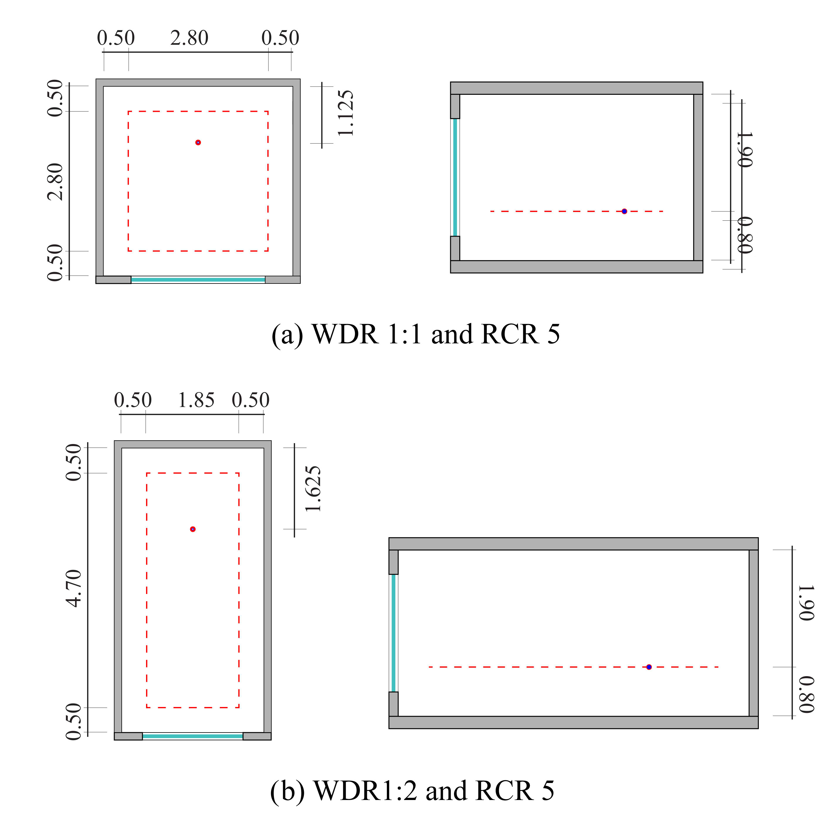
(a) and (b) Plan and section views of the room. The edge of the working plane used for the analysis further on is represented by a dashed red line; the lighting sensors are represented by a single red dot.

Fig. 1. (a) and (b) Plan and section views of the room. The edge of the working plane used for the analysis further on is represented by a dashed red line; the lighting sensors are represented by a single red dot.

Furthermore, two other characteristics of windows are investigated. The Window-to-Wall-Ratio (WWR) refers to the specific percentage of the area of the window relative to that of the room façade. WWR from 10% to 100%, in steps of 10%, are compared, as Fig. 2 illustrates. The shape of all windows is corresponding to the façade proportion. That is to say, for the rectangular façade (WDR 1:1), a rectangular shape is used for all tested windows, and for the square façade (WWR 1:2), a square shape is used for all tested windows. Then, the orientation is also analysed, so the façade where the window is placed is rotated towards the four cardinal points. To sum up, 80 design options are derived from the two WDR × one RCR × ten WWR × four cardinal points.

Figure 2

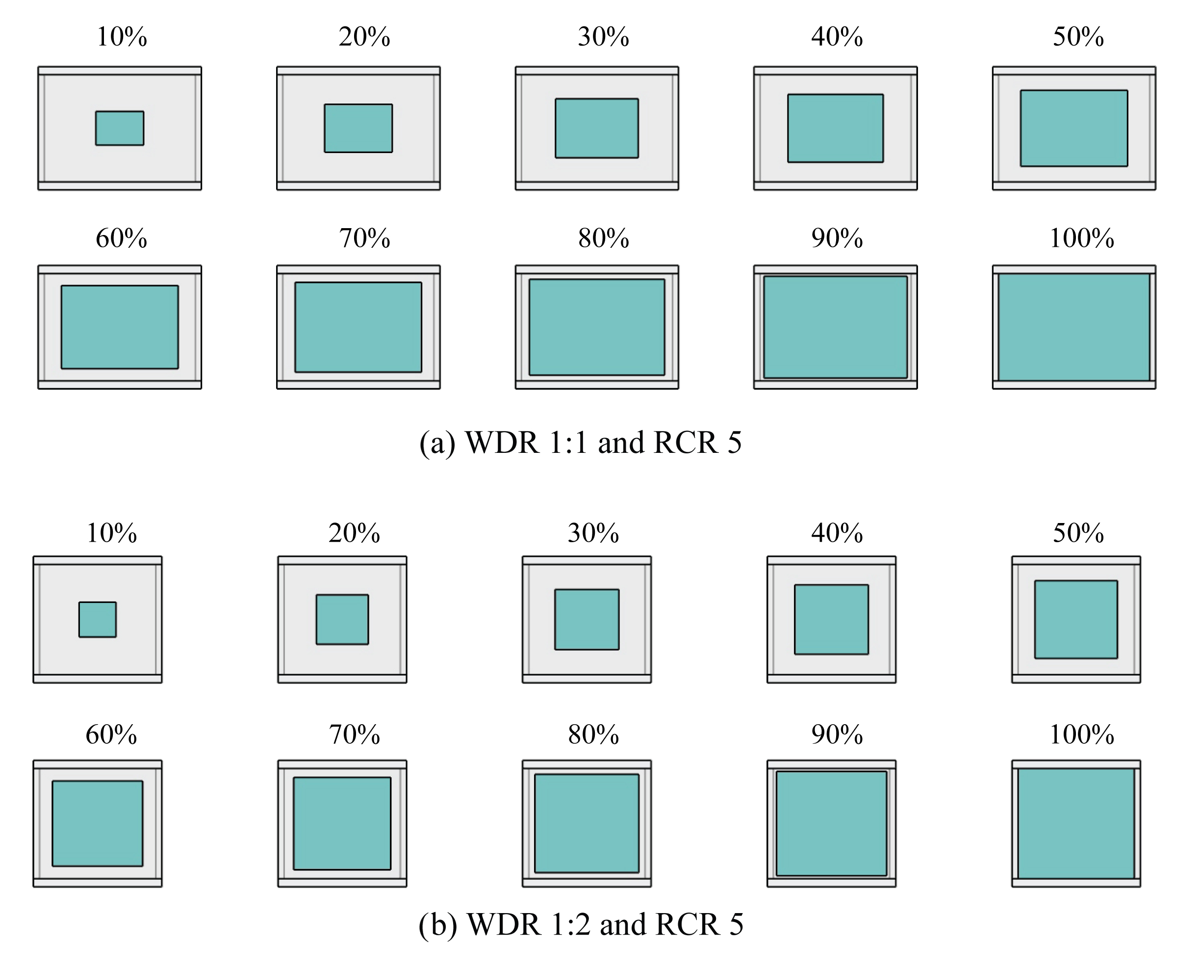
Fig. 2. (a) and (b) Façade views showing all WWR considered for comparison.

The set of 80 design options is investigated for the three representative climatic regions in Mexico [35,36]: arid, tropical, and temperate. Mexico exhibits many microclimates that are classified into three big macro climatic regions, based on the mean monthly temperature and relative humidity [36]. The three climatic regions are depicted in Fig. 3 and described below:

The arid includes the areas in the Tropic of Cancer.
The tropical, mainly warm climatic region, includes the coasts of the Pacific, Gulf of Mexico, Peninsula de Yucatan, and the Mexican Southeast in general.
The temperate climates are in the valleys of the Mexican highland, in the central areas of the country, and extended to the south of the 23^rd

Figure 3

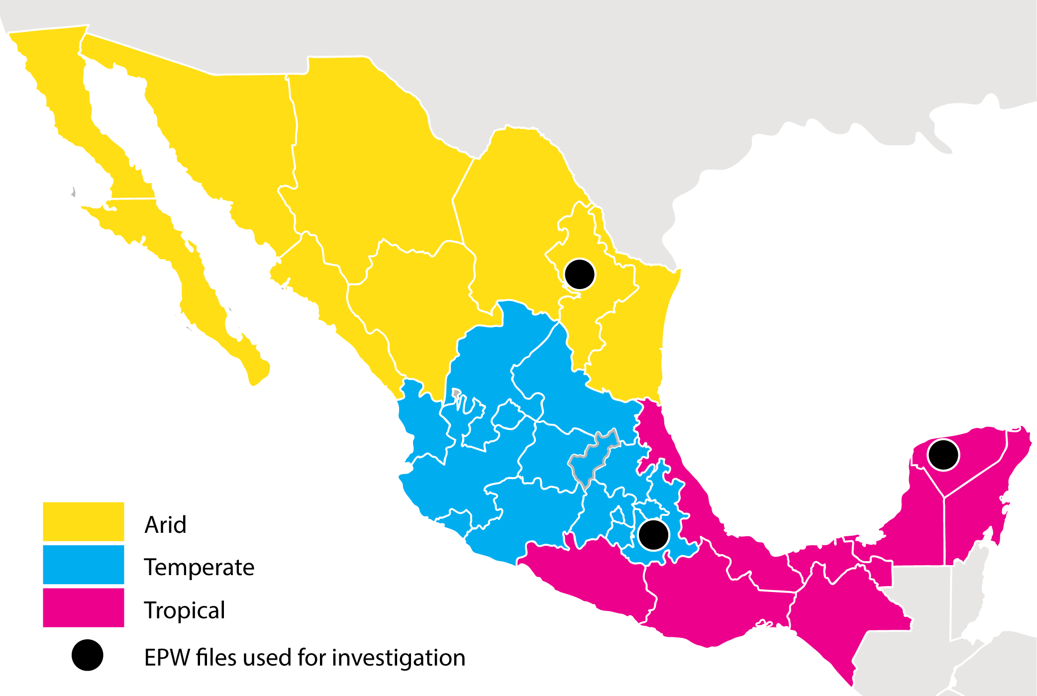
Division of climatic regions in Mexico, based on information from INEGI https://www.inegi.org.mx/temas/climatologia/ and http://atlasclimatico.unam.mx/atlas/kml/.

Fig. 3. Division of climatic regions in Mexico, based on information from INEGI https://www.inegi.org.mx/temas/climatologia/ and http://atlasclimatico.unam.mx/atlas/kml/.

Furthermore, the Mexican cities whose weather files are currently available were examined in order to prioritize those with the highest gross production in the residential construction sector for each climatic region [37]. From the examination, three cities were selected as representative of the Mexican climatic regions, so they can summarize the climate diversity of the country [35]. The EPW files of the three selected cities were finally used to run both daylight and energy simulations. Table 1 summarizes several factors derived from the three weather files. For the arid climate, the average temperature is high in summer and low in winter, while the relative humidity is around 66% almost all year long. The tropical has high temperature and medium relative humidity during summer, while medium temperature and high relative humidity during winter. The temperate region has low average temperatures (<20°) during all year long and high or medium relative humidity during summer and winter, respectively. In the end, a total of 240 models are derived from the combination of the four design variables summarized in Table 2.

Table 1

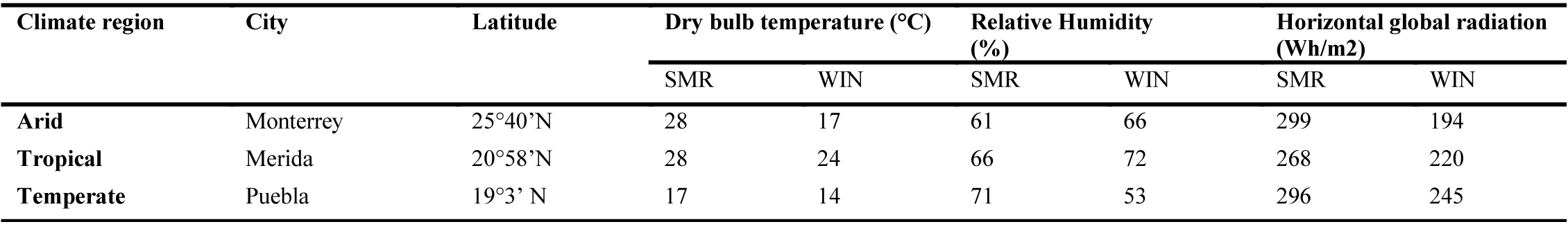
Table 1. Characteristics of the three climatic regions during summer (SMR) and winter (WIN).

Table 2

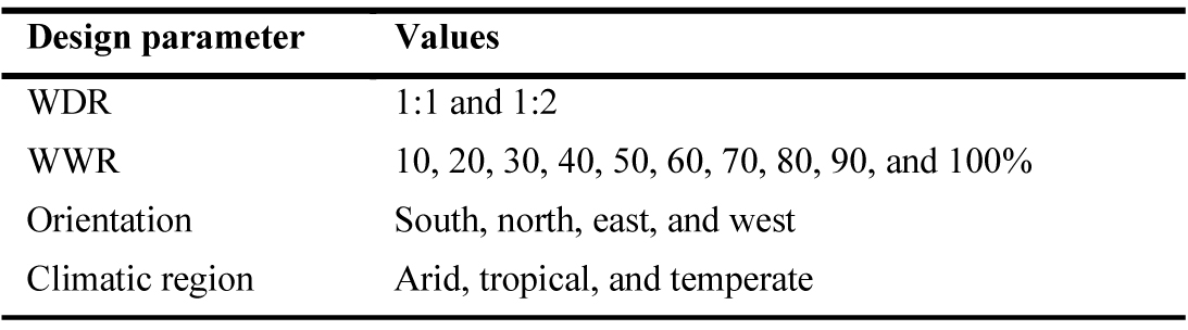
Table 2. Values for the design parameters studied.

3.2. Simulation approach

To begin this process, the room and its 240 variations are modelled with Rhinoceros according to the parameters described in Section 3.1. Then, the models are linked to Grasshopper for running the calculations with DIVA-for-Grasshoper. This software builds on thoroughly validated and tested simulation engines for daylight and building energy use – both Radiance and EnergyPlus are open source and validated by several studies [38–40]. Finally, the resulting data is statistically analysed with Minitab software. Figure 4 presents the workflow used in this study. All the steps are described below.

Figure 4

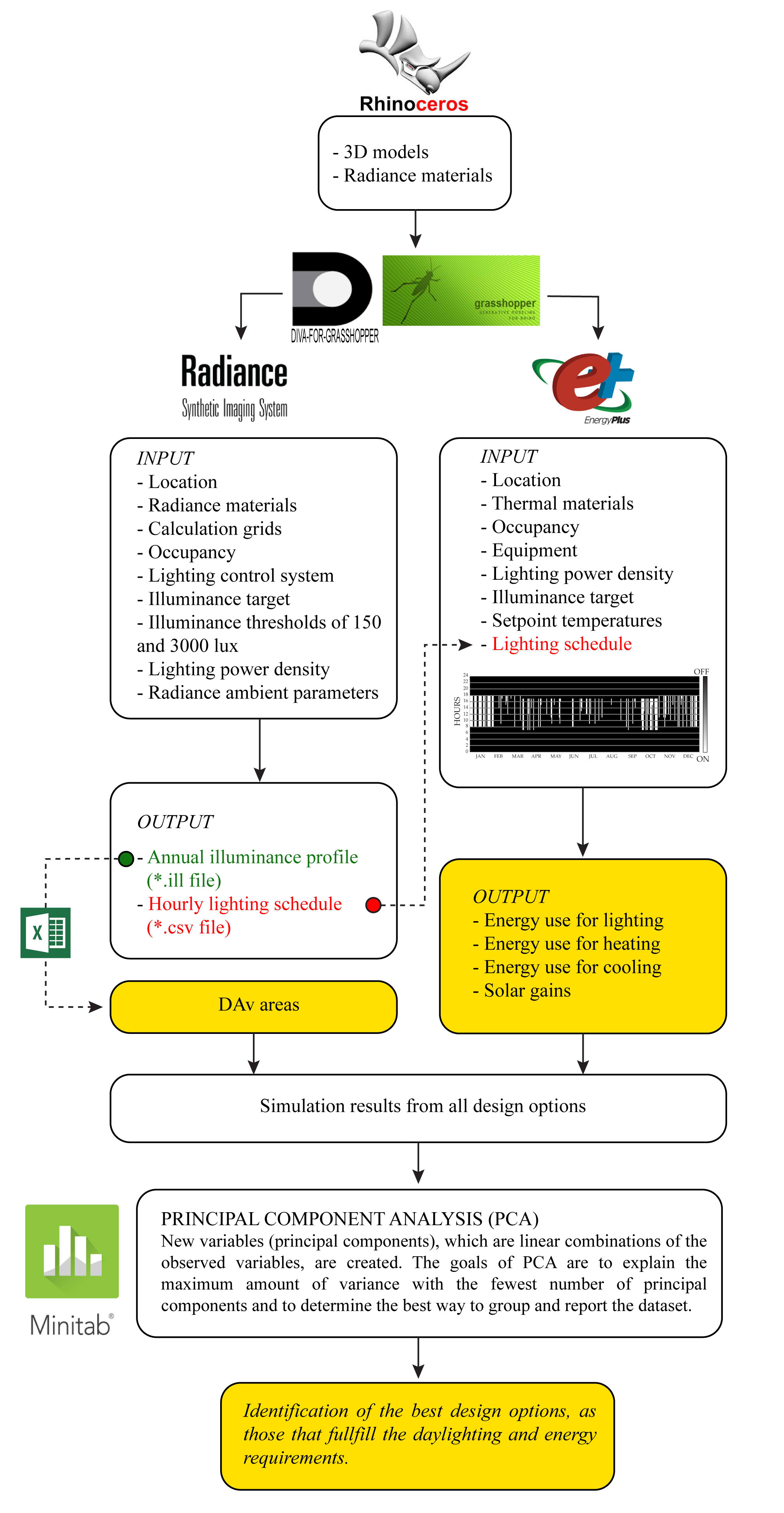
Fig. 4. Workflow for an integrated approach combining daylighting and thermal aspects through Principal Component Analysis.

Figure 5(a) illustrates the geometry used for daylight simulations run in DIVA-for-Grasshopper, which is a validated Radiance-based software that uses the Perez all-weather sky model to predict the amount of daylight in buildings, based on direct normal and diffuse horizontal irradiances from the weather files [39]. The 3D model is constructed with solids and surfaces, according to the dimensions described in Fig. 1. The materials assigned to the surfaces are characterized by 50%, 70%, and 20% reflectance for walls, ceiling, and floor, respectively. The glazing material is a 6 mm clear pane with an 88% visible transmittance. It is selected as an example of a typical glazing material used in Mexico. Table 3 summarizes the Radiance simulation parameters that were set after running a convergence test.

Figure 5

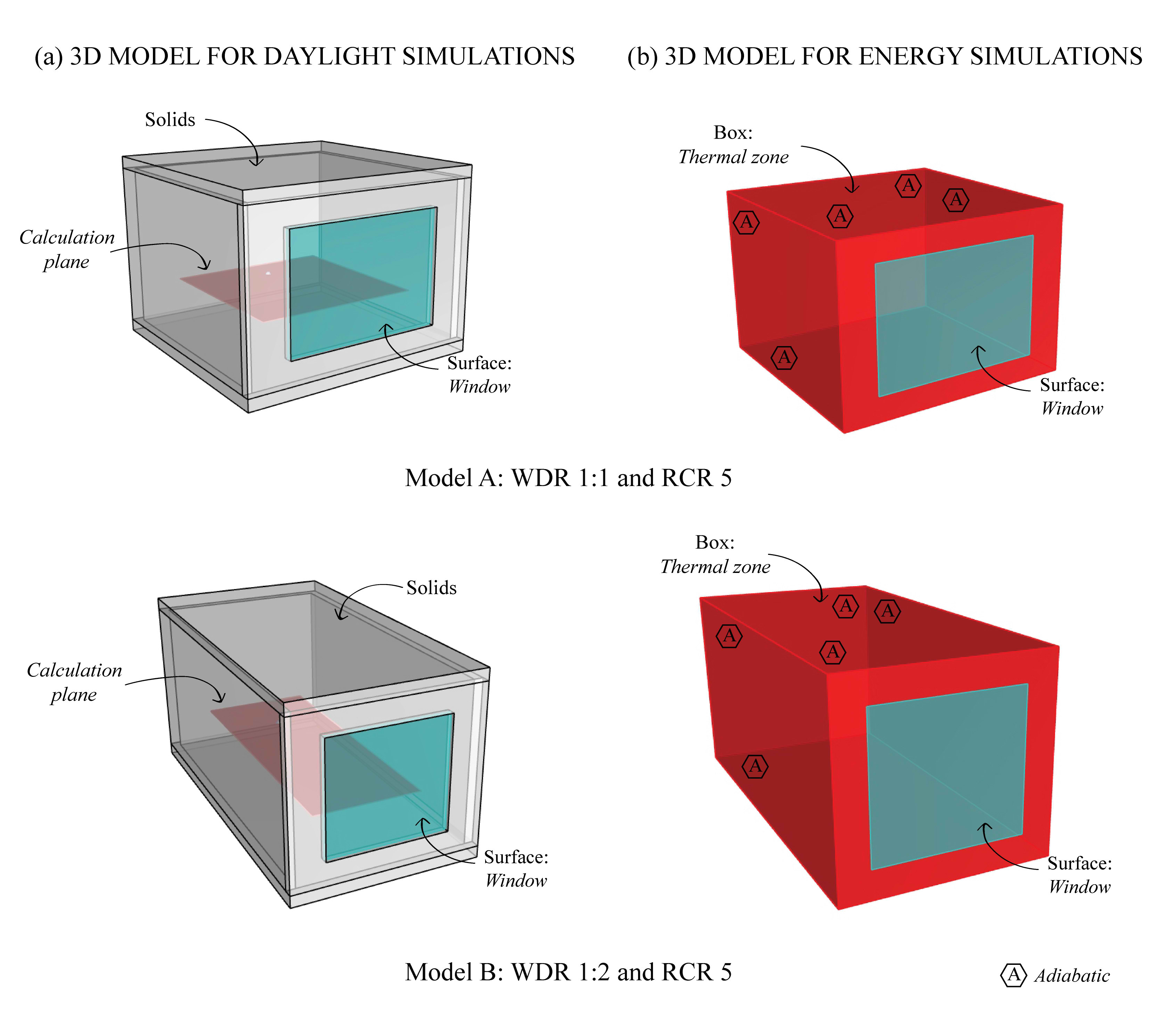
Fig. 5. 3D model constructed for: (a) daylight simulations, and (b) energy simulations.

Table 3

Table 3. Radiance ambient parameters.

Sensor points for the daylight calculations are placed inside the room, 0.25 m apart, over a horizontal plane that runs at a 0.50 m distance from the room perimeter and 0.80 m from the floor, as shown in Figs. 1 and 5(a). A lighting sensor is located in the middle of the back section of the calculation plane. It is used to run the electric lighting control analysis by using a photosensor dimming source, based on Radiance backward raytracing. The illuminance target is set to 250 lux, an illuminance level considered sufficient to develop the tasks usually carried out in a residential room. Surveys of residential lighting conditions consistently show levels that are lower than recommended practice – e.g. median illuminance at seating location 120 lx, versus IES recommendation of 300 lux [4,41–43].

Either the working day of the residents or the occupancy patterns of residential spaces have the quality of being very changeable. Nevertheless, the architectural space is something that will never change unless the surrounding urban environment changes [19]. Therefore, considering the annual hours when it is daylight is very practical to understand the full daylight potential derived from architectural design. Thus, this work considers all daylit hours during the year for the DDM calculation.

To meet the requirements for energy simulations, the 3D model has to be modified. Figure 5(b) illustrates the geometry used for energy calculations in EnergyPlus, a thermal simulation program thoroughly validated and tested in practice to assess the energy performance of conventional building systems [44]. Basically, the zone component is created by using a box where the window rectangle is overlapped to one vertical surface.

In Mexico, 95% of households do not have thermal insulation and 85% of houses that are located in hot regions do not possess thermal insulation; their comfort level is maintained by air conditioning, which consumes much energy [36]. The main construction materials for walls and roofs are block, brick, stone, and concrete, according to housing censuses conducted by the INEGI [37]. The selection of the construction materials is not necessary linked to the climatic region. In fact, most of the Mexican standards related to the performance of the thermal enclosure in buildings are voluntary.

Because this work is not focused on the different construction materials and their thermal properties, but rather focuses on the effect of daylight and solar gains through windows, a simplification of the thermal model is carried out. Except for the façade where the window is placed, the thermal transmittance from all walls, ceiling, and floor are set to be adiabatic. Furthermore, the main façade is characterized by a fixed generic material from the EnergyPlus database. This approach is particularly useful because the data obtained from daylight, solar gains, and energy calculations can be mainly an indication of the variations in the design options here studied. Then, solar gains could be included in the final heat balance equations. Several researchers have utilised similar simplifications to reduce bias from the different construction materials in order to focus on specific measurements [45,46].

The glazing system is characterized by a U-value of 5.894 W/m²-K and a 0.905 SHGC. The heating and cooling setpoints are 20°C and 24°C, respectively. The occupancy and equipment loads are 0.05 people/m² and 7.3 W/m² with a home-schedule (full occupancy at night and partial at daytime). The lighting energy calculation is based on the output of DIVA simulation results, but with an extended time from 6 h to 22 h to better fit with the conventional schedule use of a residence. A 10.6 W/m² lighting power density is also established.

3.3. Performance indicators

Climate-Based Daylight Modelling (CBDM) is used in this study to obtain the annual illuminance profiles, which consist of the time-series of predictions per point evaluated over a horizontal workplane, usually hourly for a full year [47]. Thus, realistic sun and sky conditions are employed in the simulations and the resulting datasets contain the extremes in the luminous environment that are typically encountered in actual buildings under real sky conditions. In this paper, the CBDM metric used for evaluations is the Daylight Availability (DAv), which is founded on the Useful Daylight Illuminance (UDI) metric [48,49]. Through DAv, the working plane is divided into four portions, each achieving a specific target of illuminance, during a certain percent of the time. The four areas are described below:

Actual fully daylit: This area is reported when useful illuminances (300 – 3000 lux) are over 50% of the yearly analysis period during the daylit hours. This area also includes the illuminances over 3000 lux when they do not reach 5% of the time.

Actual partially daylit: This area is measured when supplemental illuminances (150 – 300 lux) are met, but they do not reach either the non-daylit or the actual fully daylit area.
Non-daylit: This area is reported when daylight illuminances fall under 150 lux for at least 50% of the yearly analysis period.
- Over lit: This area is measured when daylight illuminances exceed the maximum threshold of 3000 lux for more than 5% of the daylit hours. This area might signify a potential for glare and heat gain [50,51].

For this investigation, the actual fully and actual partially daylit areas are considered sufficient to develop common visual and manual tasks with ease, especially for residences where a wide range of ages has to be considered.

As regards the annual energy performance, it is estimated from the Total Annual Energy (TAE) used on-site to supply the artificial lighting, heating, and cooling energy systems, all normalized by floor area (kWh/m²). The solar gains, namely the ‘windows total transmitted solar radiation energy’, are also accounted for. Solar gains refer to the short-wave solar radiation transmission through the external windows. Like the other energy loads, solar gains are normalized by floor area (kWh/m²).

Table 4 summarizes all performance indicators. Some of them should be maximized (↑) whereas others minimized (↓) to get the best overall performance and to find a balance between daylight provision and solar protection.

Table 4

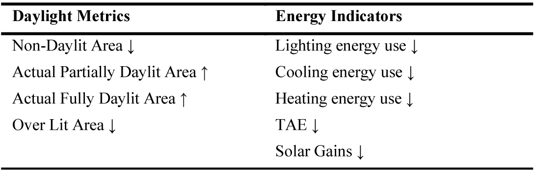
Table 4. Performance indicators used for evaluation.

3.4. Principal component analysis

The methodology employed in this work is based on the Principal Components Analysis (PCA), which is a multivariate statistical technique, widely used by almost all scientific disciplines [52–55]. It is a technique for reducing the dimensionality of large datasets, increasing interpretability but at the same time minimizing information loss [54]. PCA can also be applied to describe the data in terms of new variables or principal components, so that, trends can be visualized and correlations among the variables can be depicted.

Hence, PCA represents the pattern of similarity of the observations and the variables by displaying them as points in maps [56]. Its goal is to extract the important information from the data table and to express this information as a set of new orthogonal variables called ‘principal components’. PCA is used in this work to organize all daylight and energy results from the 240 design options around two main axes. It is also used to find strong relationships in the derived dataset and to determine the best way to group and report it.

In brief, the original data are plotted on a new coordinate system with an X-axis and a Y-axis. These axes are related to the eigenvalues and eigenvectors of the covariance matrix. In PCA, the eigenvalues (also called characteristic values or latent roots) are the variances of the principal components and each eigenvector is a unit vector pointing in the direction of a new coordinate axis. Then, the axis with the highest eigenvalue is the axis that explains the most variation [54,56,57]. The main steps followed when performing PCA evaluations are the following:

Standardization of the range of the continuous initial variables so that each one of them contributes equally to the analysis. This can be done by subtracting the mean and dividing by the standard deviation for each value of each variable. Thus, all the variables are transformed to the same scale.

\[ z=\frac{value-mean}{standard\ deviation} \]

Covariance matrix computation: PCA provides a data table, in which observations are described by several new uncorrelated variables that maximize variance [56]. The data matrix summarizes the correlations between all the possible pairs of variables, that is to say, how much the pairs of variables change together. The formula of the covariance is:

\[ Cov\ \left(X,Y\right)=\sum\frac{(xi-x̄)(y_i-ȳ)}{n-1} \]

where:

x_i = data value of x

y_i = data value of y

x̄ = mean of the variable X

ȳ = mean of the variable Y

n = number of data values

* If positive, then the two variables increase or decrease together (correlated)

* If negative, then one increases when the other decreases (inversely correlated)

Eigenvectors and eigenvalues: They are linear algebra concepts that are computed from the covariance matrix to determine the principal components of the data. Every eigenvector has an eigenvalue, and their number is equal to the number of dimensions of the data. In this paper, for an 8-dimensional data set, there are 8 variables, therefore there are 8 eigenvectors with 8 corresponding eigenvalues. The eigenvectors of the covariance matrix are actually the directions of the axes where there is the most variance (most information) and that are the principal components. Besides, eigenvalues are simply the coefficients attached to eigenvectors, which give the amount of variance carried in each principal component. By ranking the eigenvectors in order of their eigenvalues, highest to lowest, it is possible to get the principal components in order of significance. After having the principal components, to compute the percentage of variance (information) accounted for by each component, a division of the eigenvalue of each component by the sum of eigenvalues is made. Thus, the percentage of the variance of the data (proportion) is obtained.
Feature vector: The components with higher significance (feature vectors) can be kept and the components with lesser significance discarded. This last step will reduce dimensionality. However, if the aim is to describe the data in terms of new variables (principal components) that are uncorrelated without seeking to reduce dimensionality, leaving out lesser significant components is not needed. More information about PCA could be founded in [16,17].

4. Results and discussion

The following section reports the statistical findings of the research, focusing on the optimal window configurations for the three climatic regions. In addition, design guidelines and the derived targets for daylighting metrics and solar gains are also included in this section. Original data from simulations are available at Mendeley Data [58].

4.1. Experiment results

The statistical analysis is based on the results from the daylight and energy simulations from the 240 design options. The following metrics are computed: the actual fully daylit area plus the actual partially daylit area, the non-daylit and over lit areas, as well as solar gains and the lighting, heating, cooling, and TAE uses. A PCA is run to reduce the number of variables, to make the data easier to analyse, and to find the best way to group and report the dataset. Table 5 shows that the first principal component (PC1) accounts for 58% of the total variance; moreover, PC1 plus the second principal component (PC2) account for 80.1%; meanwhile, the first four principal components explain 97.3% of the variation in the data.

Table 5

Table 5. Eigenanalysis of the Correlation Matrix.

Table 6 presents the correlations among the nine metrics. The variables that positively correlate the most with PC1 are the actual fully + partially daylit areas (0.385), and the lighting energy use (0.279). Instead, PC1 inversely correlates the most with the over lit area (-0.435) and solar gains (-0.426). Therefore, increasing values of the actual daylit areas and the lighting energy use increases the value of PC1, whereas increasing values of the over lit area and solar gains decreases the value of PC1.

Table 6

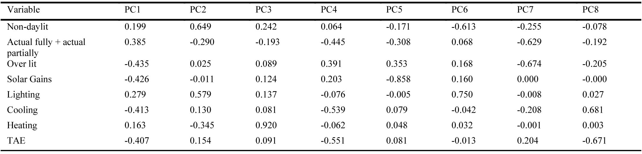
Table 6. Eigenvectors.

As regards PC2, the non-daylit area (0.649) and the lighting energy use (0.579) are the variables that positively correlate the most with it. On the contrary, PC2 inversely correlates the most with the heating energy use (-0.345) and the actual fully + partially daylit areas (-0.29). Hence, increasing values of the non-daylit area and the lighting energy use increases the value of PC2, whereas increasing values of the actual daylit areas and the heating energy use decreases the value of PC2.

The loading plot in Fig. 6(a) depicts the results for the first two components, PC1, and PC2. It is visually revealing which variables have the largest effect on each component. Loadings can range from -1 to 1. Loadings close to -1 or 1 indicate that the variable strongly influences the component. Loadings close to 0 indicate that the variable has a weak influence on the component. To summarize, PC1 is positively correlated with the actual fully, partially daylit and non-daylit areas, as well as with the lighting and heating energy uses. Nevertheless, PC1 is inversely correlated with the overlit area, solar gains, cooling energy use, and TAE. As regards PC2, it is inversely correlated with the actual fully and partially daylit areas, as well as with the heating energy use, whereas it is positively correlated with the other metrics.

Figure 6

Daylighting and energy indicators: (a) Loading plot, and (b) Score plot with 240 dots, each representing a single model. The optimal quadrant (IV) is highlighted with a dotted edge.

Fig. 6. Daylighting and energy indicators: (a) Loading plot, and (b) Score plot with 240 dots, each representing a single model. The optimal quadrant (IV) is highlighted with a dotted edge.

What is interesting about the loading and score plots in Figs. 6(a) and (b) is that they allow clustering all 240 design options into four different quadrants, so the correlations among the metrics can be identified. At first sight, quadrant I (+,+) is strongly related to the lighting and non-daylit area, while quadrant II (-,+) is strongly related to the overlit area, TAE, and the cooling energy use. Besides, quadrant III (-,-) is only related to the solar gains, and quadrant IV (+,-) is related to the actual fully and partially daylit areas, as well as with the heating energy use. As a result, the window configurations can be correlated with the specific metrics within each quadrant.

The most surprising correlation of the TAE is with the cooling energy use: both metrics are strongly and negatively correlated with PC1 (quadrant II (-,+)). Instead, the lighting and heating energy loads are positively related to PC1 (quadrants I (+,+) and IV (+,-), respectively). In reviewing the literature, no data was found on the association between increasing the use of cooling energy use in particular climates by introducing daylight into the space. On the contrary, reducing the use of electrical lighting has been the general intent in many projects and certification systems [21].

It can also be inferred from the chart, that the optimal design options are those enclosed within the quadrant IV (+,-), which has been highlighted in Fig. 6(b). This quadrant is positively correlated with proper lighting levels whereas it is negatively correlated with the annual energy loads. Thus, all dots within quadrant IV match up the optimal solutions, that is to say, the optimal window configurations.

To better interpret the trends, all design options are clustered by the space design parameters in Fig. 7. Hence, it is observed that the temperate climate is the one with the most number of models correlated with the actual fully + partially daylit areas. On the contrary, the tropical is the climate with less number of models within the quadrant IV (+,-). It is also observed that the WDR 1:1 gets higher values for those metrics within the quadrant IV (+,-). Besides, the quadrant I (+,+) only includes models with WDR 1:2.

Figure 7

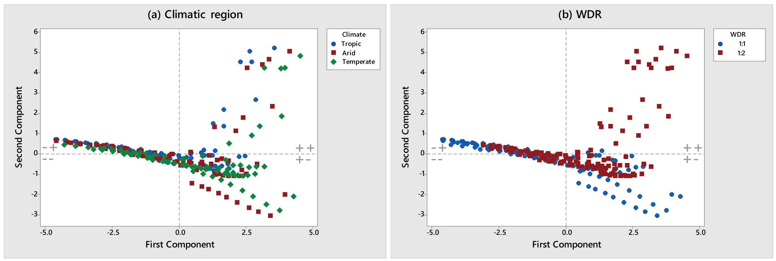
Fig. 7. Score plot of the simulation results, grouped by the two space design characteristics: (a) Climatic region and (b) WDR.

Furthermore, all results are clustered by the two window design parameters in Fig. 8. Thus, it is observed that the north orientation is the best suited, followed by the west. Only a few models oriented towards east and south are within the quadrant IV. Besides, most of the models with WWR 30-60% are distributed within the quadrant IV. Data from this figure can be compared with the data in Fig. 7 which shows a clear relation between WWR and the other design variables. That is to say, the room and the window design characteristics are related to each other. Overall, specific criteria can be derived from the optimal combinations clustered within quadrant IV (See Section 4.3).

Figure 8

Fig. 8. Score plot of the simulation results, grouped by the two window design parameters: (a) Orientation and (b) WWR.

4.2. Linking the daylight availability with the energy use

Due to space limitations, the results from the non-optimal models have been omitted and only the results for the optimal cases are presented in this section. The dataset with the 240 design options is included in a spreadsheet that can be downloaded from the Mendeley Data [58]. An insight into the optimal and non-optimal results is displayed in the Appendix A.1.

Figure 9 summarizes the daylight simulation results from the optimal models identified with the PCA, namely those within the quadrant IV. Then, the main advantages regarding the daylight availability can be depicted from the statistical analysis. First, it should be pointed out, there is no consensus yet as to what should be the target values for the daylit areas or the occurrence of any of the daylit illuminances [50]. Thus, the investigation here presented is exploratory in nature.

Figure 9

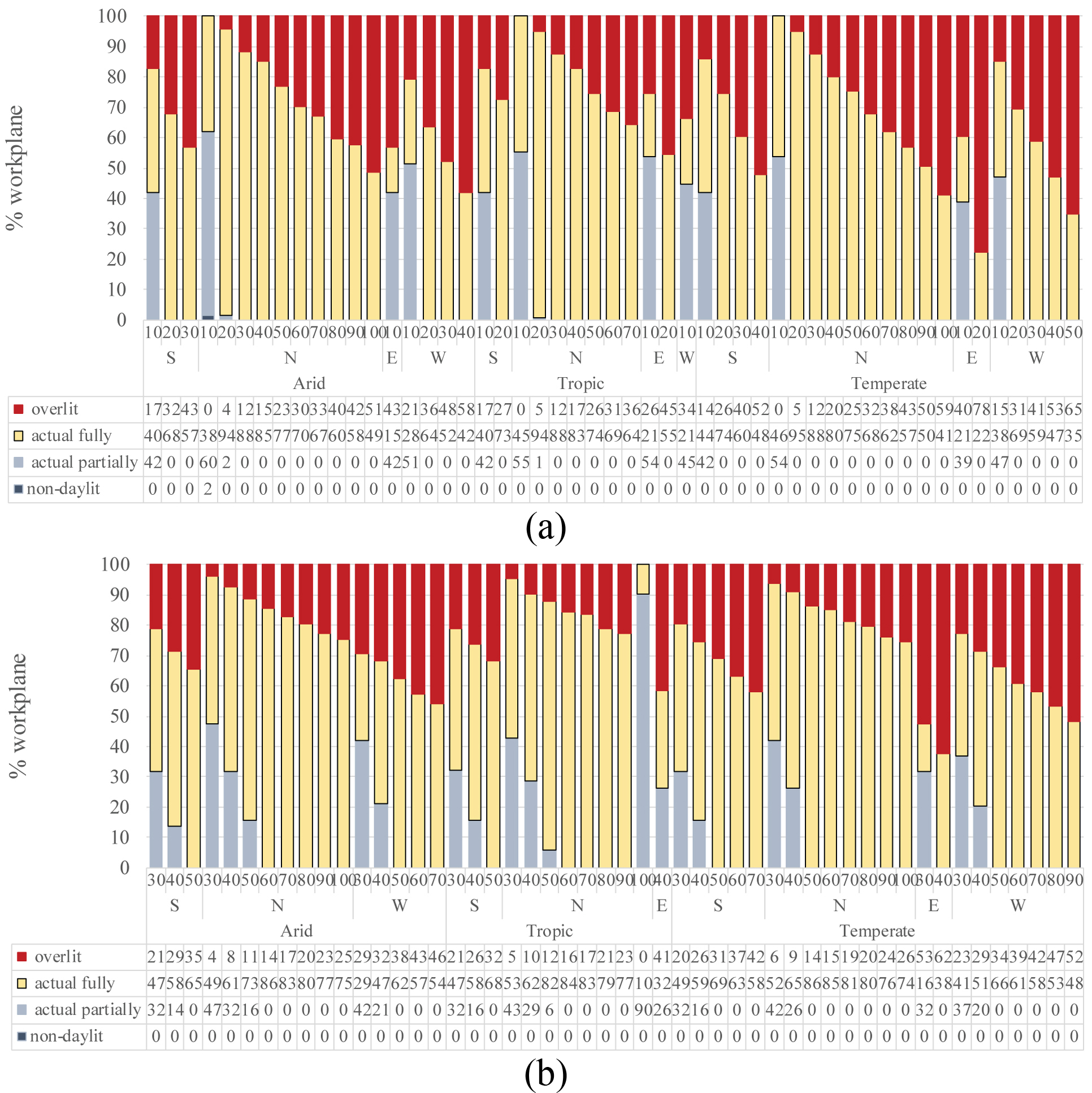
Fig. 9. Results from daylight simulations: Optimal design options according to WWR, orientation, and location for: (a) WDR 1:1, and (b) WDR 1:2.

The primary discernment to identify the best-case scenarios involves the following objectives:

Avoid the excessive illuminances, related to glare and thermal discomfort, so the over lit area should be less than 100%.
Provide useful illuminances for visual tasks in residential spaces, so the non-daylit area should be less than 50%.

Further descriptive analysis in Fig. 9 shows that the optimal design options from the PCA properly achieve both targets. However, a few cases seem to provide results unusually small or large for the actual daylit (sum of the actual fully + the actual partially) and over lit areas. For example, the case with WDR 1:1, WWR 20% facing towards East at the temperate climate, that achieves a daylit area of 22% and an over lit area of 78%. The few outliers like this one are linked to the thermal results: the statistical variances for the energy indicators (e.g. solar gains and cooling energy use) are much lower for the outliers/optimal cases than those for the non-optimal (e.g. the mentioned outlier achieves 177 kWh/m² for cooling whereas the worst-case scenario achieves 578 kWh/m² in a temperate climate).

The specific objective of this study is to balance proper daylighting levels (actual daylit areas) with thermal and energy implications. Therefore, potential relationships between the actual daylit areas and TAE, as well as between the over lit area and the cooling energy use, are explored through scatterplots. Figure 10 displays all optimal design options for pairs of variables at their (x,y) coordinates. Three main scatterplots are presented – each corresponds to a specific climatic region.

Figure 10

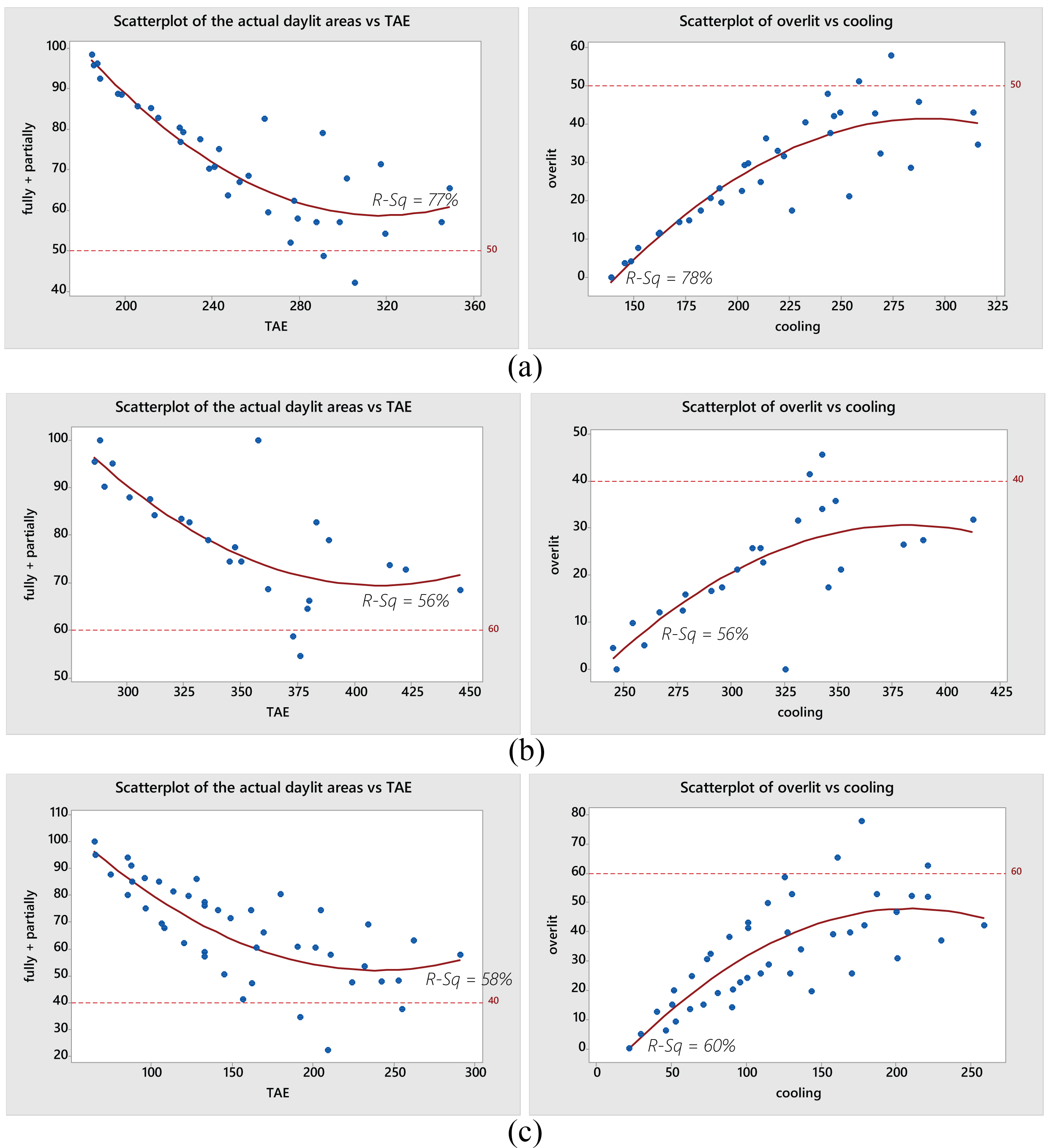
Scatterplots displaying the optimal design options for: (a) arid climate, (b) tropical climate, and (c) temperate climate. The curves display the regression fit.

Fig. 10. Scatterplots displaying the optimal design options for: (a) arid climate, (b) tropical climate, and (c) temperate climate. The curves display the regression fit.

Figure 10(a) shows that, for the arid region, most of the optimal configurations get more than 50% of the workplane as actual daylit area (sum of the actual fully + the actual partially), and less than 50% as over lit area. Only two outliers are identified. They correspond to the model with WWR 100% and WDR 1:1 at the north that gets 49% and 51% for the two mentioned areas. Besides, the model with WWR 40% and WDR 1:1 at west that gets 42% and 58% for the two related areas. Regarding the energy implications, both outliers achieve comparatively low values for TAE and cooling energy use.

Regarding the tropical region, Fig. 10(b) indicates that most of the optimal configurations get more than 60% of the workplane as actual daylit area (or as the sum of the actual fully + the actual partially daylit areas) and less than 40% as over lit area. The two exceptions were two models oriented towards the east, namely, the one with WDR 1:1 and WWR 20%, and the one with WDR 1:2 and WWR 40%. These last two models get an actual daylit area of 55% and 58%, respectively, and an over lit area of 45% and 41%, respectively. As regards the energy implications, both outliers reach comparatively low values for TAE and cooling energy use.

As regards the temperate region, Fig. 10(c) shows that most of the optimal configurations achieve more than 40% as actual daylit area and less than 60% as over lit area. Only three outliers are identified. Two of them are models with WDR 1:1: one with a WWR 20% at east, and the second with a WWR 50% at west. These two models achieve 22% and 35% as actual daylit areas. Moreover, they achieve 78% and 65% as over lit areas. The third exception was the model with WDR 1:2 and WWR 40% at East, which gets 38% as actual daylit area and 62% as over lit area. All these cases achieve comparatively low values for TAE and cooling energy use.

To summarize, the cause of the outliers has been determined. Although they get low energy loads, their daylight provision is not appropriate enough. Thus, further analysis and the main findings can be conducted without them.

Table 7 summarizes the general targets derived from the PCA and the scatterplots. One reference was the US Green Building Council’s LEED system, which specifies that a key performance indicator for daylight is the overall percentage of regularly occupied zones within a building that is “daylit”. Particularly, LEED V.4 requires to demonstrate through annual computer simulations that spatial Daylight Autonomy of 300 lux during 50% of at least 55% or 75% of the occupied floor area is achieved [59]. Another reference was the requirement suggested in [48], according to daylit area evaluations – the Daylight Autonomy of 150 lux during 50% can be considered a good simulation-based metric to mimic the partially daylit areas. However, the mentioned references are generally applied with no consideration regarding the climate site. Besides, in another work [51], it was concluded that the overlit area should be confined to a range of 40% to 50% according to the building orientation. This last recommendation was focused on only a particular climate.

Table 7

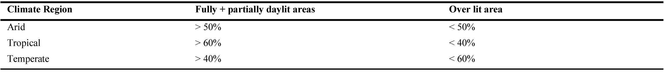
Table 7. Target limits for the DAv areas, according to the climate site.

Therefore, specific targets should be proposed for specific climate regions. In this work, a range of 40% to 60% of the occupied floor area was proposed as the reference goal. The range was derived from the statistical analysis – the targets correspond to areas for which either the majority or a sizable portion of the design configurations achieved the design goals. The remaining design configurations were non-optimal. From here, it is concluded that the climate must be considered as a determinant factor when establishing the target limits for the actual daylit and over lit areas.

Table 7 indicates that the temperate climate is particularly able to endure high levels for the over lit area (up to 60%). This could be related to its low temperature (<20°C) all year long (Refer to Table 1). In contrast, the tropical climate, which has high temperatures all year long (around 28°C during summer and 24°C during winter) tends to tolerate low levels for the over lit area (up to 40%). As regards the arid climate, which has high temperature during summer (~28°C) but low temperature during winter (17°C), can tolerate moderate levels for the over lit area (up to 50%).

Therefore, it is clearly a strong relationship between the daylight illuminances (quantified within the over lit area) and the energy use. Hence, it is confirmed that daylight, though always associated with solar gains, is also helpful to save energy, particularly for the thermal conditioning systems. These results provide a new insight that relates the actual daylit and over lit areas with specific climate conditions.

Figure 11 illustrates the energy results for the optimal design options derived from the PCA. Therefore, the main advantages of their energy performance can be identified. This last, considering as the best-case scenarios in every climate region, the models that:

Achieve the highest saving percentages for solar gains, cooling energy use, and TAE.

Figure 11

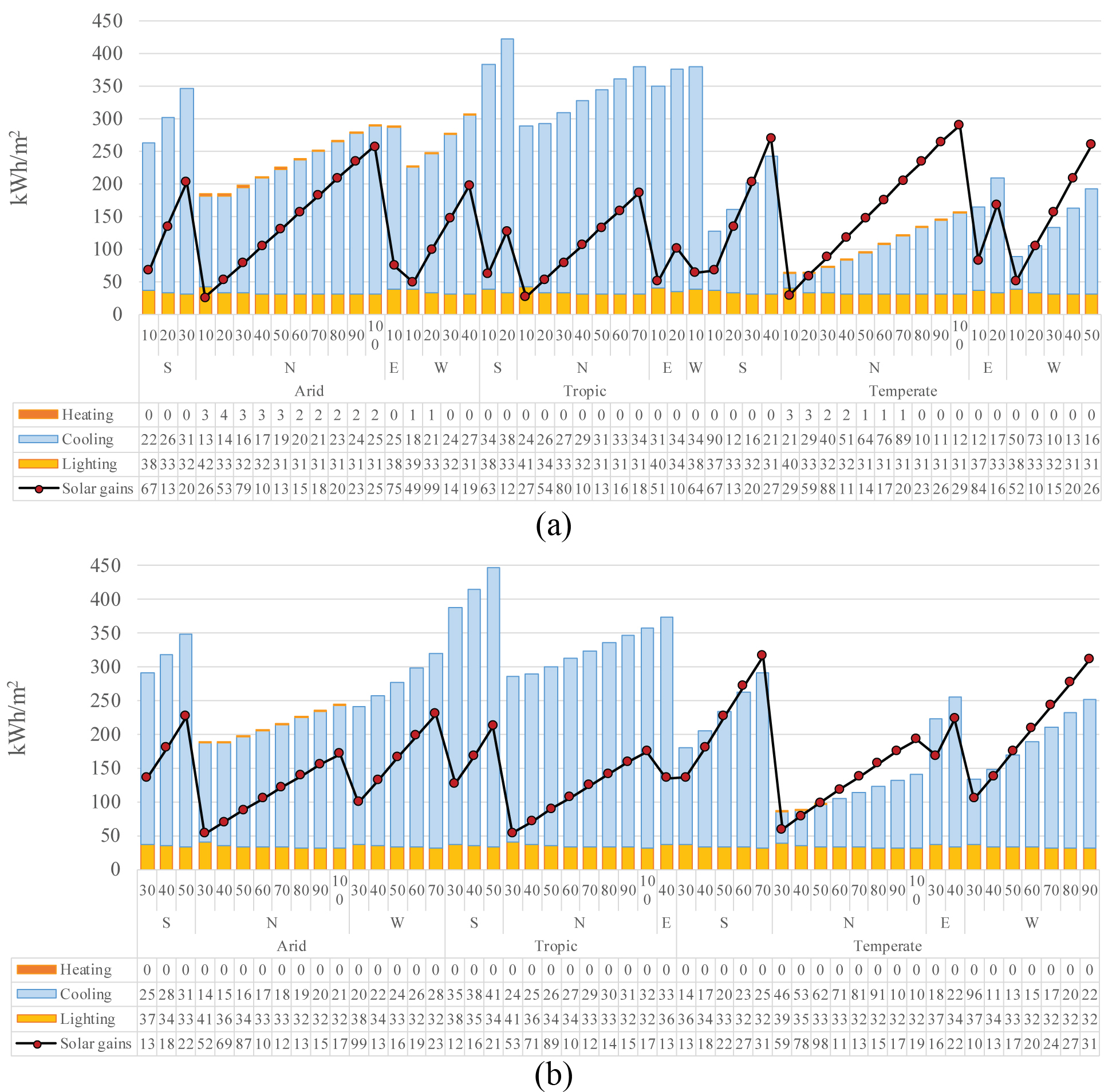
Fig. 11. Results from energy simulations: Optimal design options according to WWR, orientation, and location for: (a) WDR1:1 and (b) WDR 1:2.

The energy savings are obtained from the percent error (ε%) for each energy indicator, for each design configuration. ε% is the relative difference between an energy value obtained from the worst-case scenario and the corresponding energy value obtained from a particular design configuration. Hence, the worst-case scenarios, in every climate region, were the models that achieved the highest solar gains, cooling energy use, and TAE. They are established as the 100% possible energy consumption, so that, the ε% is obtained with the following equation:

\[ \varepsilon \%=\frac{EnergyResult_{WorstCaseScenario}-EnergyResult_{Design\ option}}{EnergyResult_{WorstCaseScenario}} \]

All the case scenarios can be accessed from the dataset [58].

Regarding the arid climate, the model characterized by a WDR 1:1, a WWR 100%, and oriented towards the east, represents the worst-case scenario. It achieves the highest solar gains of 748 kWh/m², as well as the highest energy use for cooling and TAE rising at 675 kWh/m² and 706 kWh/m², respectively. Nevertheless, the optimal models within the quadrant IV get solar gains lower than 258 kWh/m². Moreover, their lighting, cooling, and heating energy uses are kept less than 42 kWh/m², 316 kWh/m², and 4 kWh/m², respectively. As a result, the TAE for the optimal models is lower than 349 kWh/m². Hence, considerable improvements can be accomplished from an appropriate design in the arid region, for instance, a ~50% energy reduction, compared to the worst-case scenario.

As regards the tropical climate, the worst-case model is the one with a WDR 1:1, a WWR 100%, and oriented towards the west. It achieves the highest values for solar gains, cooling energy use, and TAE in this region, rising 638 kWh/m², 728 kWh/m^2, and 759 kWh/m², respectively. Contrary to the optimal models within the quadrant IV, whose solar gains are less than 212 kWh/m². Besides, the lighting and cooling energy uses from these models remain below 41 kWh/m², and 412 kWh/m², respectively. The heating energy use is not necessary for the tropical region. Therefore, the TAE is less than 446 kWh/m² for this climate, meaning a ~40% energy savings in comparison to the worst-case.

For the temperate climate, the worst-case scenario is characterized by a WDR 1:1, WWR 100%, and oriented towards the east. It reaches solar gains of 829 kWh/m², cooling energy use of 578 kWh/m², and TAE of 608 kWh/m². Instead, the optimal design options achieve solar gains lower than 315 kWh/m². Besides, their lighting, cooling, and heating energy uses remain below 40 kWh/m², 259 kWh/m², and 3 kWh/m², respectively. Thus, the TAE is kept lower than 291 kWh/m², saving energy by a ~50%.

4.3. Design guidelines

General findings are deduced when comparing models with similar design characteristics. In the case of models with different WDR, but the same climate, orientation, and WWR, the following observations. From Fig. 9, it is observed that the sum of the two actual daylit areas is higher for those models with WDR 1:2 than for those with WDR 1:1. Then, the over lit area remains much lower for a WDR 1:2 than for a WDR 1:1. From Fig. 11, it is noticed that all energy indicators remain lower for a WDR 1:2 than for a WDR 1:1. It can thus be suggested that deep rooms have the best overall performance.

Regarding the WWR, specific recommendations are identified for every orientation at each climate region. Table 8 summarizes the optimal values for the design parameters. It could be used as Guidelines to find the appropriate design parameters that are relevant to the climates. To complement the information provided in the Guidelines, a Configurations Matrix with all the 240 design options is included in Appendix A.2. Both the Guidelines and the Configurations Matrix allow building designers to visualize the performance of the optimal design configurations.

Table 8

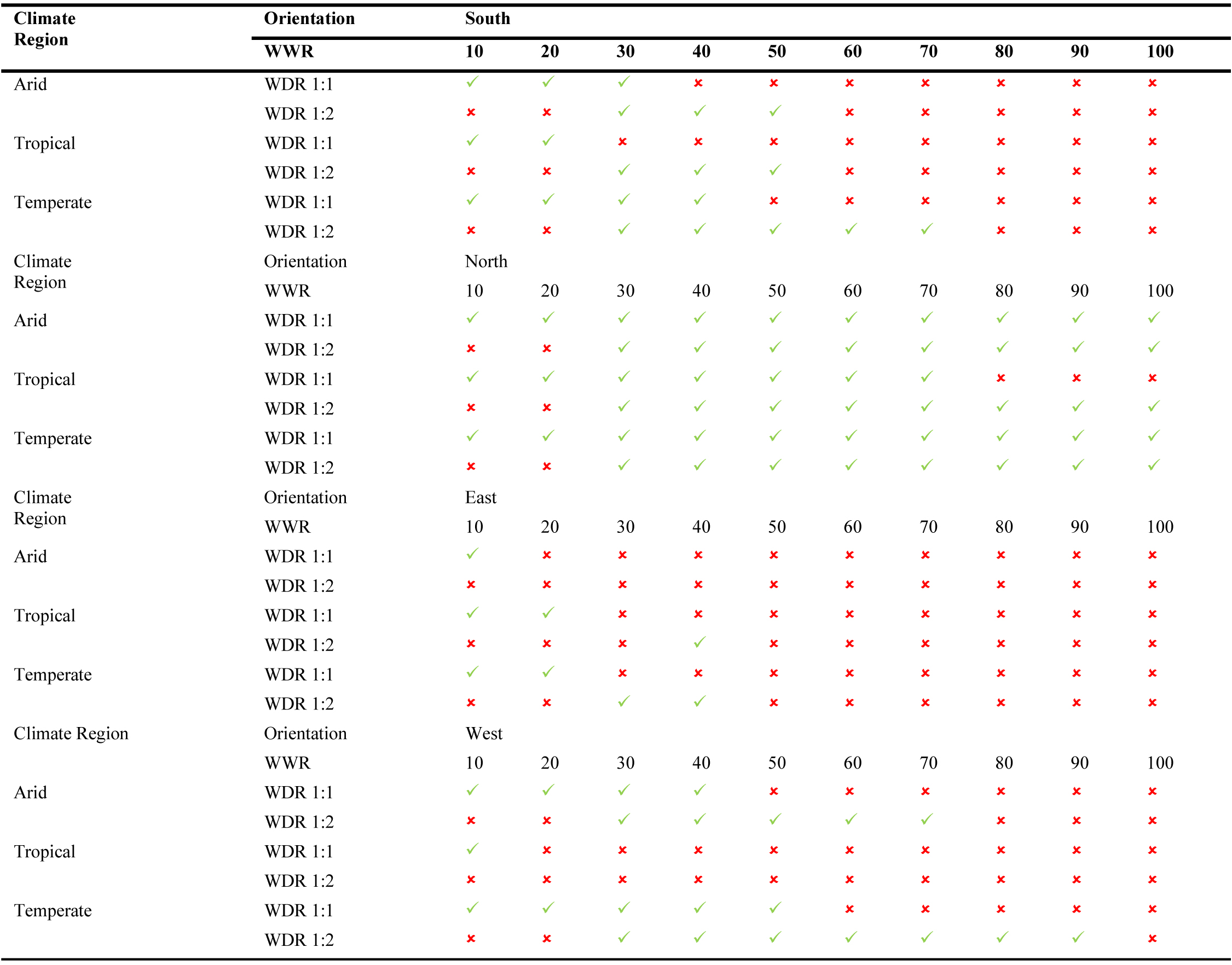
Table 8. Guidelines for designing windows according to the climate region and room depth: optimal (✓) and non-optimal (×).

Regarding the south orientation, the general guideline is that smaller WWR are better suited for shallow rooms (WDR 1:1) than for deep rooms (WDR 1:2), in the three climates. For the north orientation, most WWR are optimal at all climates since this is the façade less exposed to the solar trajectory at the northern latitudes. For shallow rooms, all WWR are recommendable, except for the largest (WWR 80-100%) at the tropical. For deep rooms, smaller windows (WWR 10-20%) are not recommendable in any climate whereas WWR 30-100% are favourable in the three regions.

As regards the east orientation, only a few WWR are optimal for shallow rooms. That is to say, WWR 10% in the arid region, and WWR 10-20% in the tropical and temperate climates. For deep rooms, only a WWR 40% is recommendable for the tropical climate as well as WWR 30-40% for the temperate region.

For the west orientation, the general guideline is similar to that for the south. That is to say, smaller WWR are better suited for shallow rooms than for deep rooms, but only in the arid and temperate climates. Instead, a WWR 10% is the only one found favourable for a WDR 1:1 located in the tropical.

The recommendations for the east and west orientations are not equivalent due to the impact of the seasonal cloud cover, which is different in the three cities. As an indication, sun-paths in Fig. 12 depicts the direct normal illuminance during the daylit hours of the solstices and equinoxes at the three cities. Thus, it is possible to support that the arid climate presents much cloudier sky conditions during the afternoon than during the morning, mostly in summer. Then, the tropical presents much cloudier sky conditions during morning hours, all year long. Finally, the temperate climate presents a more pronounced cloud cover during the afternoon than during the morning, all year long.

Figure 12

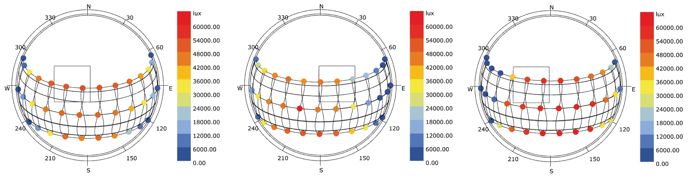
Sun-path diagrams showing the hourly data scored (a) arid climate, (b) tropic climate, (c) temperature climate during four representative days (summer solstice, equinoxes, and winter solstice): Direct Normal Illuminance (lux).

Fig. 12. Sun-path diagrams showing the hourly data scored (a) arid climate, (b) tropic climate, (c) temperature climate during four representative days (summer solstice, equinoxes, and winter solstice): Direct Normal Illuminance (lux).

5. Conclusions

This paper investigated and compared the outcomes of many window configurations for residential spaces. The effect of choosing a shallow or a depth room, a big or a small window, the orientation of the openings, and all these variables according to specific climatic regions, showed to be key elements when studying the performance of building spaces. These findings complement those of earlier studies that were focused on studying one factor at a time without linking-up with other design variables or with the climatic factors. Currently, very scarce studies had been focused on proposing design guidelines for specific climate regions.

This study came from an integrated approach combining several space design characteristics with a coupled daylighting and energy evaluation. In brief, two WDR, ten WWR, four orientations, and three different climates were simultaneously analysed through a statistical technique widely used by almost all scientific disciplines. Essentially, PCA allowed comparing all 240 design configurations derived from the combination of the four design variables. Besides, PCA permitted extracting the most important information from simulation results in terms of finding a balance between the daylight availability and the thermal assessment.

Besides, the loading and score plots allow showing all results clustered into four quadrants. Hence, the fourth was optimal since it was positively and strongly correlated with high levels of the actual daylit areas (fully plus partially). Instead, it was inversely correlated with high levels of solar gains and TAE (total energy used on-site for lighting, cooling, and heating). In the end, PCA was a useful tool to specify design guidelines for each climate region, namely the arid, tropical, and temperate. One main finding was that deep rooms are better suited than shallow rooms in terms of the overall balanced performance, at the three studied climates. Contrary to expectations, this study finds that introducing daylighting into the space did not contribute to reducing the total energy use (although it contributes to reducing the lighting energy). Instead, cooling energy use resulted in the most significant load for TAE.

Furthermore, specific WWR were recommended for deep or shallow rooms, according to every orientation at each climate. Generally, for the south orientation, smaller windows were better suited for shallow rooms than for deep rooms, in the three climates. For the west orientation, smaller windows had a better overall performance in the arid and temperate climates. As regards the north orientation, almost all WWR were optimal. In contrast, for the east orientation, only a few WWR were in good agreement with a balanced solution. The resulting design guidelines will be of interest to architects and designers when working on project specifications.

From above, a profound analysis of the seasonal cloud cover was advantageous to understand the particularities of every climate and its effect on the design guidelines proposed to find a balance between daylight provision and thermal issues. Since daylight is always associated with solar gains, it was also pointed out that the climate is a key element when establishing the target limits for the actual daylit areas and the over-lit areas. For instance, particular climatic conditions, such as temperature during summer and winter, must be considered when proposing guidelines and targets for climate-based daylighting metrics.

To summarize, some climates as the temperate were able to endure higher levels for the over lit area (up to 60%). On the contrary, arid and tropical climates tolerate lower levels for the over lit area (up to 50% and 40%, respectively). These results were in good agreement with the statement that excessive illuminances (accounted within the over lit area) have been correlated with thermal discomfort. The targets proposed in this work are a first and new insight that relates the over lit area with specific climate conditions. These findings may help the research community and certification systems when looking for specific targets applied to sustainable buildings.

To conclude, PCA was successfully set as the basis of a methodology that could help architects and consultants to define design strategies for specific locations and climates that further lead to updating high-performance standards in buildings at regional levels. Thus, this study is a starting point into criteria considerations, so it can be extended to investigate other types of climates and additional building components (e.g. glazing and construction materials). Further research should also consider shading devices, such as blinds, complex fenestration systems, or improved glazing, to regulate solar radiation, daylight levels, and energy consumption. A potential future study should take into account other objectives and criteria, such as view quality, acoustics, and glare, together with solar gains, energy consumption, and daylight provision.

Appendix A: An insight into the results from all the design options

A.1. Scatterplots of the results from all the 240 design configurations

The purpose of the scatterplots included in the main document was to show the relationship between the metrics accounted for the optimal designs – how the metrics increase or decrease by changing some design variables. The non-optimal designs were not included since their results were not necessarily related to the metrics analysed in the scatterplots. However, their inclusion may be useful to show the general trends derived from the full dataset and to corroborate the relations with the optimal-case scenarios. These last were defined as those that achieve the following design goals:

Avoid the excessive illuminances, related to glare and thermal discomfort, so the over lit area should be less than 100%.
Provide useful illuminances for visual tasks in residential spaces, so the non-daylit area should be less than 50%.
Achieve the highest saving percentages for solar gains, cooling energy use, and TAE.

Figure A.1 includes the results for the temperate region, both the optimal and non-optimal. As observed from these graphs, some outliers (non-optimal designs) were included within the proper percentages for the metrics. Let’s take design option 131 as an example. From the left part of Fig. A.1, it seems that it achieved proper levels for both the overlit area and the cooling energy use. From the right part of Fig. A.1, it seems that it is barely reaching 40% for the actual daylit areas with low energy consumption. However, the two graphs were focused only on the mentioned metrics.

Figure A.1

Scatterplots of the actual daylit areas vs TAE, and of the overlit area vs cooling energy use. The full set of design options for the temperate region has been included. The curves display the regression fit. Data labels (numbers) were included to help the reader to identify the design configurations.

Fig. 13. Scatterplots of the actual daylit areas vs TAE, and of the overlit area vs cooling energy use. The full set of design options for the temperate region has been included. The curves display the regression fit. Data labels (numbers) were included to help the reader to identify the design configurations.

Figure A.2 is plotted to better understand the overall results. Here, design option 131 was non-optimal since it did not provide useful illuminances for visual tasks. That is to say, the non-daylit area exceeded the target limit of <50% workplane. Consequently, it was one of the design options with the highest lighting energy use. As mentioned in the paper, daylight is also effective on health and well-being of occupants (apart from providing light to the eyes and contributing to saving energy).

Figure A.2

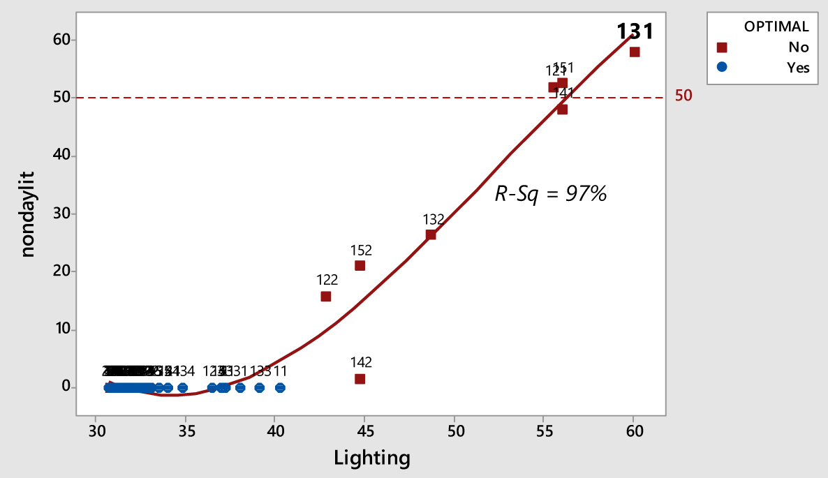
Scatterplot of the nondaylit vs lighting. The full set of design options for the temperate region has been included. The curve displays the regression fit. Data labels (numbers) were included to help the reader to identify the design configurations.

Fig. 14. Scatterplot of the nondaylit vs lighting. The full set of design options for the temperate region has been included. The curve displays the regression fit. Data labels (numbers) were included to help the reader to identify the design configurations.

This type of analysis could be developed for each of the outliers. However, they were omitted due to space limitations. The dataset with the 240 design options is included in a spreadsheet that can be downloaded from the Mendeley Data [58].

A.2. Configurations Matrix for all the 240 design configurations

To complement the information provided in the guidelines (See Table 8 in Section 4.3), a Configurations Matrix with all the 240 design options is here presented in Fig. A.3. The aim is to allow the performance comparison between the optimal and non-optimal options. Specifically, two metrics are displayed:

fully + partially daylit areas: % workplane that achieves illuminances in the range 150-3000 lux, during at least 50% of the occupied hours).
TAE: cooling + heating + lighting = total annual energy use.

Figure A.3

Configurations matrix for both optimal and non-optimal design configurations. The optimum solutions are highlighted with the squares. For interpretation of the references to colour in this figure, please refer to the web version.

Fig. 15. Configurations matrix for both optimal and non-optimal design configurations. The optimum solutions are highlighted with the squares. For interpretation of the references to colour in this figure, please refer to the web version.

The Configurations Matrix itself could be particularly useful for building designers to find the appropriate design parameters that are relevant to their climate. It also allows visualizing the performance of the optimal design configurations.

Acknowledgments

The author acknowledges the support of Universidad de las Americas Puebla and CONACYT.

Declaration of competing interest

The author declares that there is no conflict of interest.

References

A. Galasiu, M. Atif, R. MacDonald, Impact of window blinds on daylight-linked dimming and automatic on/off lighting controls, Solar Energy 76 (2004) 523–544. https://doi.org/10.1016/j.solener.2003.12.007
A. Pellegrino, V. Lo Verso, The energy demand for electric lighting as a consequence of different architectural building features and lighting plant characteristics, Proc. CIE 2010 Lighting Qual. Energy Effic. x035 pp. 695–703, 2010.
D.H.W. Li, A review of daylight illuminance determinations and energy implications, Appl. Energy. 87 (2010) 2109–2118. https://doi.org/10.1016/j.apenergy.2010.03.004
J.A. Veitch, J. Christoffersen, A.D. Galasiu, Daylight and View through Residential Windows : Effects on Well-being, in: Lux Eur. 2013, National Research Council of Canada, Krakow, Poland, 2013: pp. 1–6.
J. Veitch, J.A., Christoffersen, A.. Galasiu, What we know about windows and wel-being, and what we need to know, in: Proc. CIE Centen. Conf. "Towards a New Century Light., Commission Internationale de l’Eclairage, Paris, France, 2013: pp. 169–177.
M. Farley, J. Veitch, Report IRC-RR-136K. A room with a view: A review of the effects of windows on work and well-being, 2001. http://nparc.cisti-icist.nrc-cnrc.gc.ca/eng/view/fulltext/?id%BCca18fccf-3ac9-4190-92d9-dc6cbbca7a98.
P. Boyce, C. Hunter, O. Howlett, The benefits of daylight through windows, Lighting Research Center - Rensselaer Polytechnic Institute, Troy, New York, 2003. http://www.ibo.at/documents/Licht_TB07_Andersent.pdf.
J.A. Veitch, A. Galasiu, Research Report: The physiological and psychological effects of windows, daylight and view at home: Review and Research Agenda, vol. 325, 2012. https://doi.org/10.1037/e554552013-001
M.L. Persson, A. Roos, M. Wall, Influence of window size on the energy balance of low energy houses, Energy Build. 38 (2006) 181–188. https://doi.org/10.1016/j.enbuild.2005.05.006
D.H. Li, J. Lam, Evaluation of lighting performance in office buildings with daylighting controls, Energy Build. 33 (2001) 793–803. https://doi.org/10.1016/s0378-7788(01)00067-6
F. Goia, M. Haase, M. Perino, Optimizing the configuration of a façade module for office buildings by means of integrated thermal and lighting simulations in a total energy perspective, Appl. Energy. 108 (2013) 515–527. https://doi.org/10.1016/j.apenergy.2013.02.063
CIBSE, Daylighting and window design., Publicaciones IDAE, London, UK, 1999.
R. Hopkinson, P. Petherbridge, J. Longmore, Daylighting, Butterworth-Heinemann Ltd, London, 1966.
BRE (Building Research Establishment), BREEAM: the BRE environmental assessment method., (2015). www.breeam.org (accessed February 1, 2015).
International Organization for Standardization (ISO), ISO 10916:2014 Calculation of the impact of daylight utilization on the net and final energy demand for lighting, (2014). https://doi.org/10.3403/30275420u
M. Boubekri, An overview of the current state of daylight legislation, J. Hum. Environ. Syst. 7 (2004) 57–63.
Secretaría de Economía, Norma Mexicana Nmx-AA-164-SCFI-2013 Edificación Sustentable - Criterios Y Requerimientos Ambientales Mínimos, (2013) 158.
A. Nabil, J. Mardaljevic, Useful daylight illuminances: A replacement for daylight factors, Energy Build. 38 (2006) 905–913. https://doi.org/10.1016/j.enbuild.2006.03.013
C. Reinhart, J. Mardaljevic, Z. Rogers, Dynamic daylight performance metrics for sustainable building design, Leukos. 3 (2006) 7–31. https://doi.org/10.1582/leukos.2006.03.01.001
C.F. Reinhart, S. Herkel, The Simulation of annual daylight illuminance distributions-a state-of-the-art comparison of six RADIANCE-based methods, Energy Build. 32 (2000) 167–187. https://doi.org/10.1016/s0378-7788(00)00042-6
USGBC (United States Green Building Council), LEED Reference guide for building design and construction. Version 4, (2013). http://www.usgbc.org/.
E. Brembilla, D.A. Chi, C.J. Hopfe, J. Mardaljevic, Evaluation of Climate-based daylighting techniques for complex fenestration and shading systems, Energy Build. 203 (2019) 109454. https://doi.org/10.1016/j.enbuild.2019.109454
L.O. Beltrán, D.I. Liu, Evaluation of Dynamic Daylight Metrics Based on Weather, Location, Orientation and Daylight Availability, in: 35th PLEA Conf. Sustain. Archit. Urban Des. Plan. Post Carbon Cities, 2020: pp. 4–9.
L. Wen, K. Hiyama, M. Koganei, A method for creating maps of recommended window-to-wall ratios to assign appropriate default values in design performance modeling: A case study of a typical office building in Japan, Energy Build. 145 (2017) 304–317. https://doi.org/10.1016/j.enbuild.2017.04.028
A. Jakubiec, C.F. Reinhart, DIVA 2.0: Integrating daylight and thermal simulations using Rhinoceros 3D, Daysim and EnergyPlus, in: Proc. Build. Simul. 2011 12th Conf. Int. Build. Perform. Simul. Assoc., IBPSA (International Building Performance Simulation Association), Sydney, 2011: pp. 2202–2209.
C.E. Ochoa, M.B.C. Aries, E.J. van Loenen, J.L.M. Hensen, Considerations on design optimization criteria for windows providing low energy consumption and high visual comfort, Appl. Energy 95 (2012) 238–245. https://doi.org/10.1016/j.apenergy.2012.02.042
K. Alhagla, A. Mansour, R. Elbassuoni, Optimizing windows for enhancing daylighting performance and energy saving, Alexandria Eng. J. 58 (2019) 283–290. https://doi.org/10.1016/j.aej.2019.01.004
E. Ghisi, J.A. Tinker, An Ideal Window Area concept for energy efficient integration of daylight and artificial light in buildings, Build. Environ. 40 (2005) 51–61. https://doi.org/10.1016/j.buildenv.2004.04.004
I. Acosta, M.Á. Campano, J.F. Molina, Window design in architecture: Analysis of energy savings for lighting and visual comfort in residential spaces, Appl. Energy 168 (2016) 493–506. https://doi.org/10.1016/j.apenergy.2016.02.005
R.M.J. Bokel, The effect of window position and window size on the energy demand for heating, cooling and electric lighting, IBPSA 2007 - Int. Build. Perform. Simul. Assoc, 2007, pp.117–121.
J. Yu, L. Tian, C. Yang, X. Xu, J. Wang, Sensitivity analysis of energy performance for high-rise residential envelope in hot summer and cold winter zone of China, Energy Build. 64 (2013) 264–274. https://doi.org/10.1016/j.enbuild.2013.05.018
H. Peng, M. Li, S. Lou, M. He, Y. Huang, L. Wen, Investigation on spatial distribution and thermal properties of typical residential buildings in South China’s Pearl River Delta, Energy Build. 206 (2020) 109555. https://doi.org/10.1016/j.enbuild.2019.109555
CONAVI, Guía de implementación del Código de Edificación de Vivienda (CEV): Adaptación y adopción locales, 3era ed., CONAVI-SEDATU, 2017.
CIE (Commision Internationale de L’Eclairage), CIE S 017/E:2011 ILV: International lighting vocabulary, CIE, Viena, 2011.
R. Vidal-Zepeda, Las regiones climáticas de México. Temas selectos de geografía de México., UNAM, México, 2005. https://doi.org/10.14350/rig.30041
J.A. Rosas-Flores, D. Rosas-Flores, Potential energy savings and mitigation of emissions by insulation for residential buildings in Mexico, Energy Build. 209 (2020) 109698. https://doi.org/10.1016/j.enbuild.2019.109698
INEGI, Censo General de Población y Vivienda, 2014.
G. Ward, Measuring and modeling anisotropic reflection, ACM SIGGRAPH Computer Graphics 26 (1992) 265–272. https://doi.org/10.1145/142920.134078
C.F. Reinhart, J. Wienold, DIVA for Grasshopper, 2011.
DOE (U.S. Department of Energy), Energy Plus Energy Simulation Software: Weather Data, EnergyPlus, 2017. https://energyplus.net/weather (accessed June 12, 2017).
J. a. Jakubiec, G. QUek, T. Srisamranrungruang, Towards subjectivity in annual Climate-based daylight metrics, in: Proc. Build. Simul. Optim. Conf., Cambridge, MA, USA, 2016: pp. 24–31.
B. Paule, J. Boutillier, S. Pantet, Shading device control: Effective impact on daylight contribution., in: Proc. Int. Conf. Futur. Build. Dist. Sustain. from Nano to Urban Scale, Lausanne, Switzerland, 2015: pp. 241–246.
D.L. Di Laura, K.W. Houser, R.G. Mistrick, G.R. Steffy, The lighting handbook reference and application, Illuminating Engineering Society of North America New York, New York, 2011.
ASHRAE (American Society of Heating Refrigerating and Air-Conditining Engineers), ASHRE/IESNA Standard 90.1-2016. Energy standard for buildigns except low-rise residendial buildings, Atlanta, 2016.
J.O. Aguilar, J. Xamán, Y. Olazo-Gómez, I. Hernández-López, G. Becerra, O.A. Jaramillo, Thermal performance of a room with a double glazing window using glazing available in Mexican market, Appl. Therm. Eng. 119 (2017) 505–515. https://doi.org/10.1016/j.applthermaleng.2017.03.083
J. Roberto, G. Chávez, A.C. Salas, K. Angélica, G. Pardo, Evaluation of Experimental Indirect Evaporative Cooling Systems in an Extreme Hot-Humid Climate, in: 35th PLEA Conf. Sustain. Archit. Urban Des. Plan. Post Carbon Cities, PLEA, A Coruña, 2020.
J. Mardaljevic, Climate-Based Daylight Modelling, 2011. (n.d.). http://climate-based-daylighting.com/doku.php.
C. Reinhart, T. Rakha, D. Weissman, Predicting the Daylit Area — A Comparison of Students Assessments and Simulations at Eleven Schools of Architecture, Leukos 10 (2014) 193–206. https://doi.org/10.1080/15502724.2014.929007
D.A. Chi, D. Moreno, P.M. Esquivias, J. Navarro, Optimization method for perforated solar screen design to improve daylighting using orthogonal arrays and climate-based daylight modelling, J. Build. Perform. Simul. 10 (2017) 144–160. https://doi.org/10.1080/19401493.2016.1197969
J. Mardaljevic, M. Andersen, N. Roy, J. Christoffersen, Daylighting metrics: Is there a relation between Useful Daylight Illuminance and Daylight Glare Probability?, in: Proc. Build. Simul. Optim. Conf. BSO12, IBPSA, Loughborough, UK, 2012: pp. 189–196.
D.A. Chi, D. Moreno, J. Navarro, Correlating daylight availability metric with lighting , heating and cooling energy consumptions, Build. Environ. 132 (2018) 170–180. https://doi.org/10.1016/j.buildenv.2018.01.048
J. Cadima, C. J.O., M. Minhoto, Computational aspects of algorithms for variable selection in the context of principal components, Comput. Stat. Data Anal. 47 (2004) 225–236. https://doi.org/10.1016/j.csda.2003.11.001
N. Rigner, What is principal component analysis, Nat. Biotechnol. 26 (2008) 303–304. https://doi.org/10.1038/nbt0308-303
I.T. Jollife, J. Cadima, Principal component analysis: A review and recent developments, Philos. Trans. R. Soc. A Math. Phys. Eng. Sci. 374 (2016). https://doi.org/10.1098/rsta.2015.0202
H. Zou, T. Hastie, R. Tibshirani, Sparse principal components, J. Comput. Graph. Stat. 15 (2006) 262–264. https://dx.doi.org/10.1198/jcgs.2006.s7
I.T. Jolliffe, Principal component analysis, 2nd ed., Springer, New York, 2002.
Minitab 19, MINITAB. User’s Guide 2 : Data analysis and quality tools., Minitab Inc, State College, PA, USA, 2019.
D.A. Chi, [dataset] Research Data: Coupling daylighting and energy evaluations at different climate regions, Mendeley Data, V1. (2020). https://data.mendeley.com/datasets/794j77yz6h/draft?a=6ef4903b-e2b5-4476-a0c9-1e0b46c49b86. https://dx.doi.org/10.17632/794j77yz6h.1
USGBC (U.S. Green Building Council), LEED: leadership in energy and environmental design., (2015). http://www.usgbc.org/leed (accessed February 9, 2015).

Get PDF (11.3 MB)

SHARE ON