Measurement, Simulation, and Quantification of Lighting-Space Flicker Risk Levels Using Low-Cost TCS34725 Colour Sensor and IEEE 1789-2015 Standard

Sivachandran R. Perumal; Faizal Baharum

doi:10.15627/jd.2021.19

Article Outline

3. Materials and methods

4. Results and analysis

Declaration of competing interest

References

Figures and tables

Figures (21)

Tables (12)

Volume 8 Issue 2 pp. 239-254 • doi: 10.15627/jd.2021.19

Measurement, Simulation, and Quantification of Lighting-Space Flicker Risk Levels Using Low-Cost TCS34725 Colour Sensor and IEEE 1789-2015 Standard

Sivachandran R. Perumal,^* Faizal Baharum

Author affiliations

School of Housing, Building & Planning, Universiti Sains Malaysia, 11800 Pulau Pinang, Malaysia

*Corresponding author.
siva_rocks@yahoo.com (S. R. Perumal)
baharumfaizal@gmail.com (F. Baharum)

History: Received 24 April 2021 | Revised 14 June 2021 | Accepted 6 July 2021 | Published online 26 August 2021

Citation: Sivachandran R. Perumal, Faizal Baharum, Measurement, Simulation, and Quantification of Lighting-Space Flicker Risk Levels Using Low-Cost TCS34725 Colour Sensor and IEEE 1789-2015 Standard, Journal of Daylighting 8 (2021) 239-254. https://dx.doi.org/10.15627/jd.2021.19

Figures and tables

Abstract

Building owners are transitioning towards a smart lighting solution for illumination purposes. LED (Light Emitting Diode) lighting application has become a norm given its high efficacy and energy efficiencies. This paper presents an approach to monitor the percent flicker conformance of interior building lighting to international standards. The focus is on flickers induced by LED lightings. This experiment utilises a TCS34725 RGB (red, green, blue) colour sensor to measure the flicker parameters of interior lighting spaces. Light-sensitive photodiodes in the sensor detect changes in lighting intensity, and output digitised values. A Raspberry Pi4 minicomputer processes the data measured for comparison to several standards. Non-conformance is reported to building owners to take corrective actions and minimise flicker discomfort exposure to building occupants. A flicker risk level factor is determined to gauge the severity when flickers are present. This method may be used to replace luminaires or fix flickering lighting issues in buildings. The results show that the monitoring system is functional. The proposed measurement and data processing method can be incorporated into any smart building hub for automation and building performance analysis. The method may also be used to measure non-LED lighting flickers.

Keywords

Flicker, Percent flicker, Flicker index, IEEE 1978-2015

1. Introduction

Today, the notion of energy efficiencies and energy conservation measures is catalysing building owners and lighting designers to utilise LED lighting for illumination purposes. The widespread conversion to LED lighting, which yields favourable energy-saving results, has made this approach the most popular amongst other measures due to a faster capital investment return [1]. Researches on lighting and built environment primarily focus on illuminance and correlated colour temperatures. However, one of the often-overlooked lighting parameters is flicker caused by sub-par LED lighting devices. Severe flickers are noticeable by the average human eyes. In contrast, high-frequency flickers exist in almost all solid-state lightings, which is a concern to be tackled. Unaddressed flicker issues may lead to Sick Building Syndrome over time, which every organisation tend to avoid.

Lighting flickers are defined as rapid and repeated shifts in light intensity [2]. It can be graded as visually perceptible or not based on flicker frequency. Moreover, when the lighting source and the observer shift about each other, flicker occur – stroboscopic effect. Temporal Light Artefacts (TLA) are unwanted lighting effects caused by variations in light output, and flicker is a type of temporal light modulation (TLM) [3]. Humans do not detect flickers consciously, but they are processed subliminally by the average human brain. They affect visual and cognitive performance. Adverse health concerns are seen in some cases [4].

Fluorescent lighting, for example, is powered by an alternating current (AC) mains supply that varies over time (50 Hz or 60 Hz). As a result, the light output follows the same pattern to turn on and off due to the time-varying source, causing flicker. Flicker in the lighting area can cause seizures, migraines, headaches, and being visually unpleasant or constantly distracted [2]. As a result, flickers are harmful to one’s well-being.

Electrical transformers were once used to step up or down voltages to control interior lighting. The AC mains input voltages exhibit flicker characteristics due to its low frequencies – power-line flicker. Today, direct current (DC) source drives LED lighting with the advances from power electronics technology. A DC source-driver at the lighting output reduces flickering to appropriate levels, improving occupant visual comfort. The Pulse Width Modulation (PWM) technique is used to control lighting intensity levels [5]. Though lighting equipment moves toward modern LED lighting standards, source flicker can still exist at lighting ends, such as through PWMs.

This paper aims to tackle subliminal flicker by devising a lighting-space flicker detection system using a low-cost RGB colour sensor. The system alerts buildings owners when non-conformance against international flicker regulations occurs, specifically IEEE 1789-2015 standard. Moreover, the system would produce a refined risk level factor quantifying marginally-risky luminaries, which benefits buildings owners in corrective action plans. The scope of the research is to test a LED lighting-lit small room limited to a sensor unit using a minicomputer that acts as a building monitoring server. Upon successful flicker detection and risk level analysis, expansion of the system onto large building environments will be proposed, such as integration to Building Monitoring Systems. The proposed system may be used in any built environment, which has lighting systems. Figure 1 shows the steps taken to conduct this research.

Figure 1

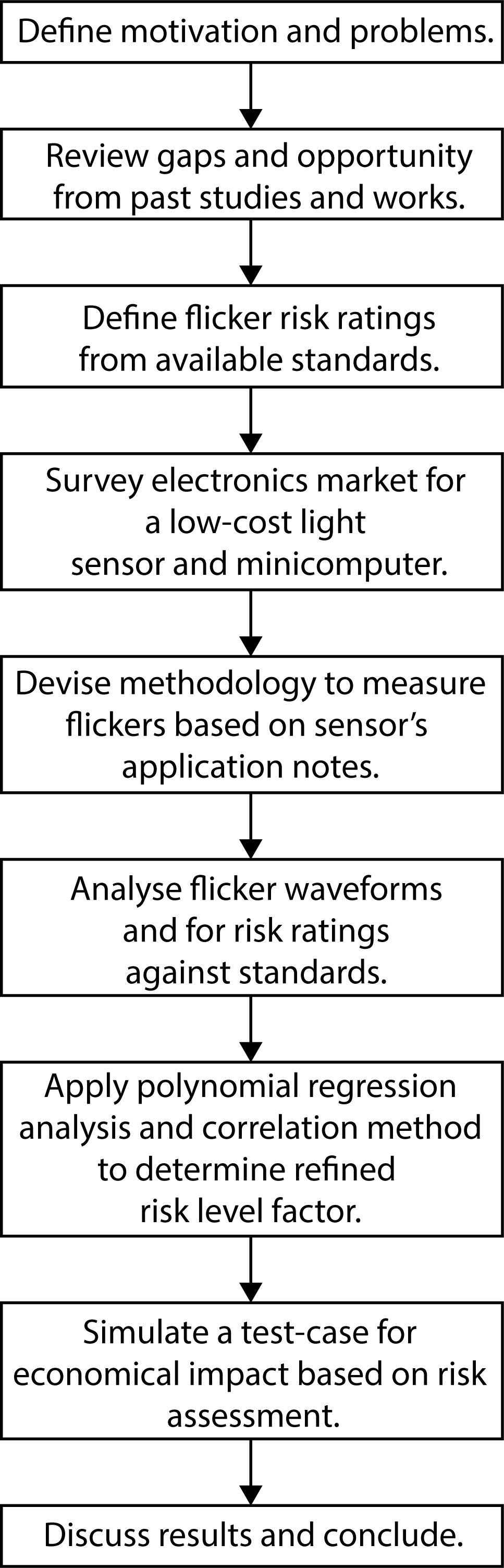
Fig. 1. Research conduction steps.

In a study to detect flickers and stroboscopic effects caused by LED lighting on a work table, the authors calculated flickers through their control parameters to simulate flickers [6]. In other words, they manipulated input parameters such as user-determined current source and lighting intensity through the Pulse Width Modulation (PWM) technique for LED lighting. Conventional lamps were simulated to produce flickers by varying input voltages. In other words, flickers were not detected through external sensors but calculated through input source data. Here, the output may not always be the same as desired inputs in practical applications, as intrinsic noises in the system may cause deviations. Lamps, albeit LED or conventional, are an open-loop system. In addition, their photometric details are usually listed in their device’s datasheet. However, low-end lighting in the markets sometimes does not come with factory measurement data.

One research noted that the appropriate parameter to measure relevant to flicker is luminous flux (lumens), but there is no standard procedure to measure them [7]. Lighting waveform flicker was manually calculated using measurement data from selenium cell (sensor) and oscilloscope readings in another research [8]. However, the researchers determined flickers from multiple single commercial LED lamp sources instead of the whole space or room. Similarly, for single lamp measurements, in another work to measure flickers, the researchers used photodiode (TSL257 sensor with additional circuitry) and oscilloscope combinations to generate flicker waveform. Fluctuations in the photodiodes’ voltage drops were plotted in the oscilloscopes and analysed [9].

Certain studies have used specific flicker measurement units such as IEC flicker meters and luminance meters [10]. However, they come in single measurement equipment and needs calibration before use. Moreover, in a built environment application, manual measurement has to be done room by room and becomes tedious. In conclusion, previous researches have shown that combining the photodiode sensor and a detection system as a whole can automate these procedures. Having a centralised system that monitors flickers and alerts building owners on the go would be beneficial when safety risk assessments are done.

2.1. Flickers in LED lighting

Today’s widespread use of LED lighting necessitates the development of new methods for assessing lighting flicker. The LED driver determines the flicker and dimming efficiency of LED lighting. Dimmers and other electronics can induce or increase lighting flicker. Lighting devices that use AC-driven LEDs are more likely to flicker. Due to inadequate filtering capacitors, DC-driven LEDs with simple or inexpensive drivers often cause systemic flickering [3,4,8]. Capacitors consume space on electronic boards. Complex electronics, such as phase-cut dimmers (triacs) and pulse width modulation (PWM) techniques, can pass on switching noise from the electronics to the lighting output in the form of flicker. Switching noise is created by high operating frequencies in Switching Mode Power Supplies (SMPS) [11].

2.2. Task performance and health issues from lighting flickers

Lighting flickers from artificial lighting can cause a variety of health problems. Neurological disorders such as epileptic seizures, headaches, nausea, blurred vision, eyestrain, and migraines are among them [1-4,8,12]. Flickers are known to reduce task efficiency and effectiveness when it comes to task execution. Studies have also linked flicker exposure to an increase in autistic behaviours, especially in children. The stroboscopic effect causes motion to appear to slow or stop. Flicker discomfort detracts from one’s well-being and efficiency at work. It can be life-threatening in severe cases [4].

When a subject is subjected to flickers for prolonged periods, the effects are exacerbated. Repeated stimulation and exposure to a retinal field in human eyes magnifies the adverse health effects [1-4]. Furthermore, the effects are stronger when the flicker source is in the middle of the field of vision since it projects to a broad region of the visual cortex, even though the flickering incident is less visible. In addition, the quanta of light influences flicker effects. High luminances in the mesopic and photopic regions produce a higher health risk [4]. When the brightness variation is high, flickers become more noticeable. Moreover, subjects are vulnerable to health issues when the contrast ratio between the flicker source and the environment is high. The flicker source’s colour contrast variance in the red light channel is considered the worst of all.

2.3. Flicker metrics

Illuminating Engineering Society of North America (IESNA) is a non-profit organisation that works on lighting standards. According to IESNA, there are two key ways to identify flickers: percent flicker and flicker index. Both metrics are defined in Eq. 1 and 2 using parameters from Fig. 2. They are older but more well-known and commonly used [7].

\[ PF=\frac{A-B}{A+B}\times100 \% \]

where PF is the percent flicker, expressed in (%), A is the maximum amplitude value of lighting waveform (max luminance), and B is the minimum amplitude value of lighting waveform (min luminance).

\[ FI=\frac{A1}{A1+A2} \]

where FI is the flicker index, A1 is the Area 1, the area above the average value as per Fig. 2, and A2 is the Area 2, the area below the average value as per Fig. 2.

Figure 2

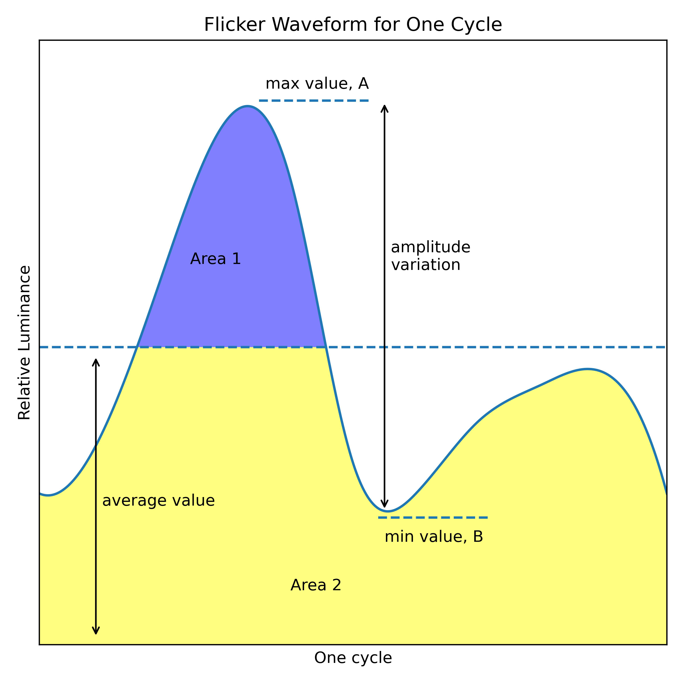
Fig. 2. Flicker waveform.

Percent flicker is measured on a 0 to 100 % scale by considering the average and peak-to-peak amplitude measurements. Amplitude refers to the lighting intensity (luminance) of the waveform. They do, however, ignore the shape, duty cycle, and frequency of the lighting waveform [4,7].

On the other hand, the flicker index is calculated on a scale of 0 to 1.0. It is a more recent formulation, but the formula is less known and used. Waveform average, peak-to-peak amplitude, shape, and duty-cycle are taken into account by the flicker index calculation as per Eq. (2). The formula, however, does not take frequency into account [4,7].

2.4. Standards on safe lighting flicker ratings

There are several newer standards and guidelines associated with flicker ratings. Amongst the properties emphasised by the newer standards are waveform modulation frequency and amplitude and waveform DC component and duty cycle.

The IEEE PAR 1789-2015 standard is the primary source of reference in this article because it breaks down the flicker ratings into three levels of risk. Having ranges of risk, particularly high-risk, low-risk, and no-risk, enables this research to generate the refined risk-level factor, quantifying marginality.

2.4.1. IEEE PAR 1789-2015

In 2008, IEEE PAR 1789 established a technical committee to assess and address solid-state lighting (SSL) flicker risk issues. LED lighting is a form of SSL. In 2012, the committee released a paper outlining a Risk Assessment protocol as a best practice [4].

The risk evaluation matrix, shown in Fig. 3, segments the effects of flickers into several risk levels. Table 1 tabulates the degree of certainty for risk level with colour saturation ranging from green to red.

Figure 3

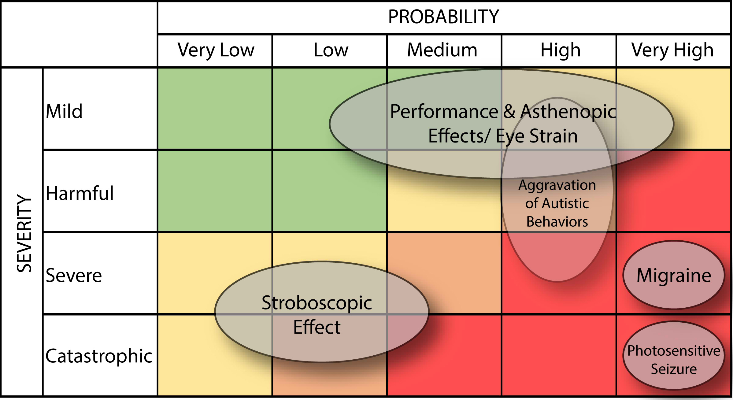
Fig. 3. IEEE 1789-2015 Risk Assessment Matrix (RAM).

Table 1

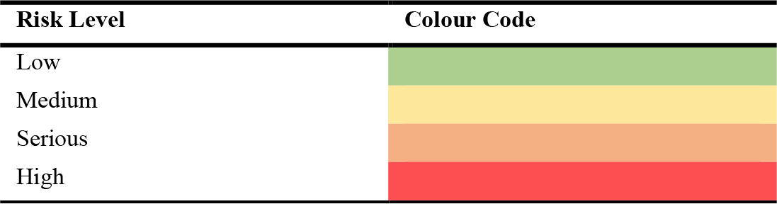
Table 1. Colour codes from IEEE 1789-2015 RAM.

Potential significant adverse health effects of flicker are mapped into the risk matrix using various sources, including reliable evidence and field expert opinions. They are represented in Fig. 3 by the oval shapes.

A selection of recommended practices is adopted based on the risk analysis performed by mapping the risk assessment matrix. Maximum flicker ratings are described mathematically using the boundary conditions between the Low-Risk and Medium-Risk zones. The boundary’s mathematical modelling is expressed in Eq. 3 [4].

\[ Max\ PF\le\ f_0\times0.08 \]

where Max PF is the maximum percent flicker, expressed in (%) and f₀ is the operating frequency of the lighting waveform (dominant fundamental frequency).

The operating frequency of an SSL product must be greater than 100 Hz to use the IEEE 1789-2015 risk assessment chart. Therefore, the product must be reviewed to ensure that it meets the application’s requirements. The maximum permissible percent flicker is calculated by multiplying the operating frequency by 0.08 and rounding the number to the nearest integer [4]. The SSL product is acceptable if the percent flicker is less than the permitted flicker. This requirement extends to the general public except for the most susceptible individuals. If obtaining an SSL’s operating frequency is difficult, the percent flicker must not exceed 10%.

A lighting waveform is further divided into three sub-levels of risk, with Eq. (3) being the maximum permissible percentage flicker. Table 2 lists them in order of risk, from no risk to low risk to high risk. Figure 4 shows the criteria in a graphical representation.

Table 2

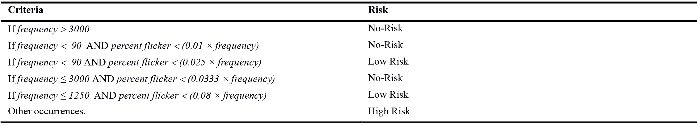
Table 2. Risk level of flicker in IEEE 1789-2015.

Figure 4

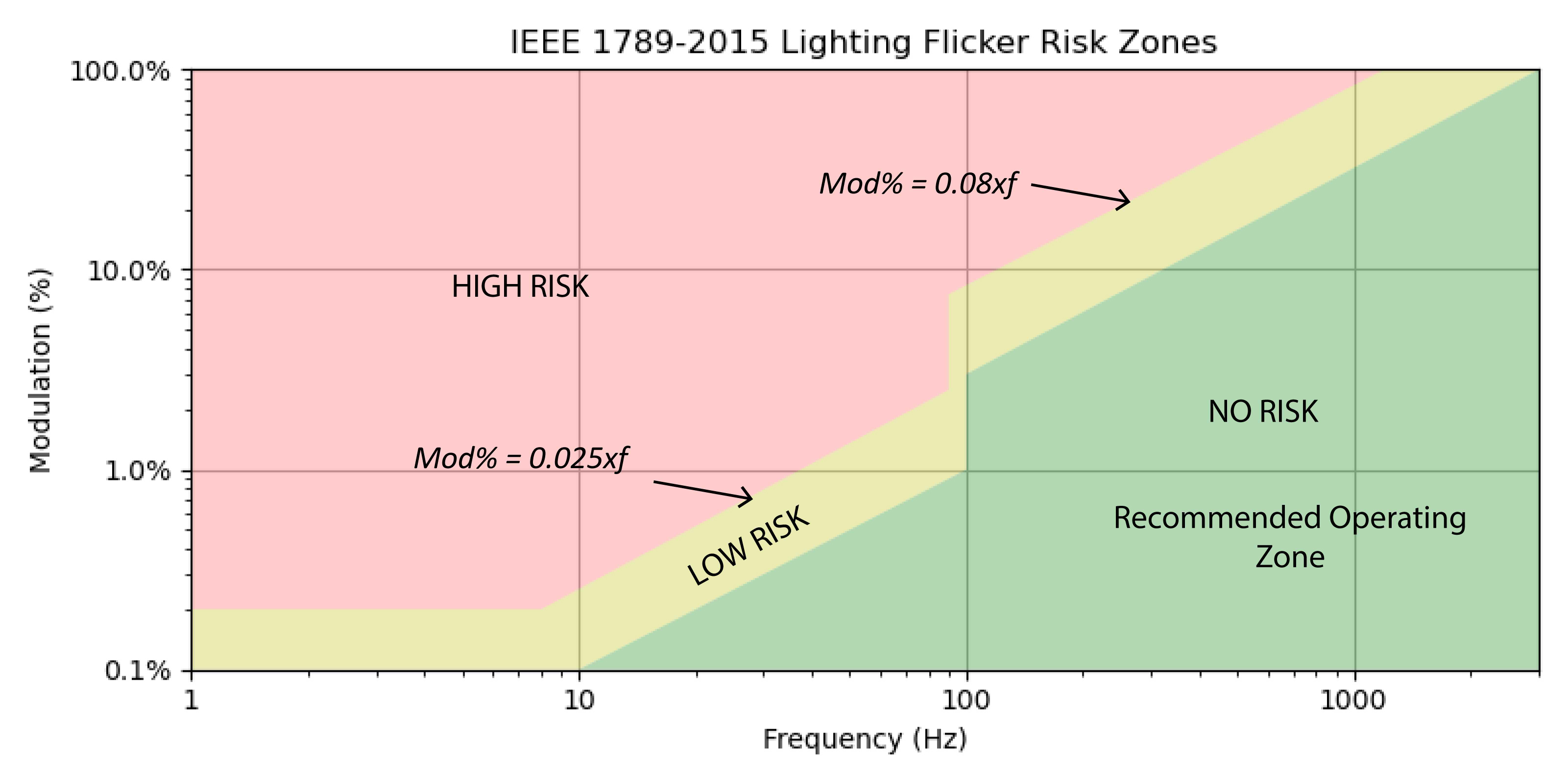
Fig. 4. IEEE 1789-2015 risk zones.

The bordering line between Low-Risk and Medium-Risk in Fig. 3 is similar to the bordering line between Low-Risk and No-Risk in Fig. 4. The boundary has been mapped into a modulation (%) and frequency graph by the IEEE 1789-2015 working group. The percent flicker of a waveform is also known as modulation (%).

2.4.2. California joint appendix 8 (JA-8.4.6 and Table-JA-8)

California Joint Appendix 8 is another standard that categorises flicker ratings of waveforms as either PASS (acceptable) or FAIL (not acceptable) [13]. In summary, JA 8.4.6 (Table-JA-8) notes that flickers are suitable to the general public for waveform frequencies greater than 200 Hz. Acceptance conditions are the same, with a percent flicker level of less than 30 %. If neither of the above conditions is met, the waveform is deemed unacceptable or unsafe. Table 3 summarises the criteria of California Joint Appendix 8.

Table 3

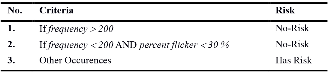
Table 3. Risk classification of JA8.

2.4.3. WELL building standard (L07 Part 2)

The flicker scores in the WELL Building Standard are identical to those in California Joint Appendix 8 [14]. If a minimum frequency of 90 Hz is exceeded at all 10% lighting output intervals from 10% to 100% light, the waveform is deemed PASS. LED products with a low-risk level of percent flicker of less than 5%, mainly when operated at less than 90 Hz, are also classified as PASS. Any other non-conforming waveform properties are considered unsafe or FAIL. Table 4 summarises the criteria.

Table 4

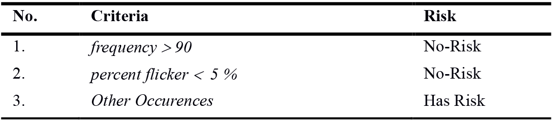
Table 4. Risk classification of WELL L07 Part 2.

2.4.4. Refined flicker risk level

IEEE 1789-2015 Standard has divided the flicker rating of lighting into three levels: no risk, low risk, and high risk. In Fig. 4, they are graded as being on the low-risk side of the medium-risk spectrum. By assigning decimal ranges to the low-risk level of the IEEE 1789-2015 table, building management teams can make more accurate decisions. Such precision is essential in facility management because those figures affect capital expenditures.

The risk level factor could be incorporated into other risk assessments by facility management teams. Risk evaluation in facility engineering can include safety, system failure, patient recovery in the healthcare industry, and many other things. A risk assessment’s findings are typically presented to management and finance teams to obtain funding. These findings are necessary because the finance department needs concrete reasons for facility overhaul plans to be approved.

If risks are present at facilities, it impacts the budgetary needs. For example, if the annual capital expenditure for building lighting maintenance is set at $1,000, multiplying by the flicker risk level factor (say, 0.321), the maintenance team is awarded an extra monetary fund of $1,000+(0.321×$1000)=$1,321 dollars. Annual capital costs for large buildings, such as factories and healthcare operations, range to millions. Thus, the few decimals figures introduced by the flicker risk level signifies thousands of dollars.

In most safety risk assessments, the likelihood (probability) and consequent (severity) variables are loosely set based on past experiences and data clustering [15]. One of the benefits of having a refined flicker risk level is that it aids in objectively breaking down the probability aspect of the risk assessment matrix’s likelihood. For example, a study on rating risk level to spacecraft orientation subsystem used an objective function to map the probability scale [16]. Furthermore, the authors objectively defined the probability scale based on spacecraft system parameters. Similarly, in another research that aims to quantify the probability scale of the risk matrix, the authors devised clear and continuous probability ranges. Their approach was through implementing a Monte Carlo simulation of single indicators, hence applying the copula model to calculate the joint risk probability of multiple indicators [17]. Finally, in a building fire risk assessment, the researchers used event tree analysis to quantify the probability scale be more definite rather than estimates [18]. Therefore, in this paper, the refined risk level or factor would further solidify risk assessments for built environments where lighting flickers concerns by objectively scaling the probability scale.

3. Materials and methods

The Lighting Flicker Monitoring system is made up of three modules. Figure 5 shows three: the sensor module, data IO (input/output) processing module, and output module. A low-cost TCS34725 RGB colour sensor makes up the sensor module. A RaspberryPi 4 (RPi4) mini computer processes the waveform data captured by the sensor module. Finally, the flicker performance of a lighting space is displayed on a monitoring screen. The results may be sent to building owners to alert them for the non-conformance of flicker performances. For this paper, the TCS34735 sensor and Raspberry Pi 4 was used. However, the choice is not limited to replicate the procedures in this methods sections using other devices.

Figure 5

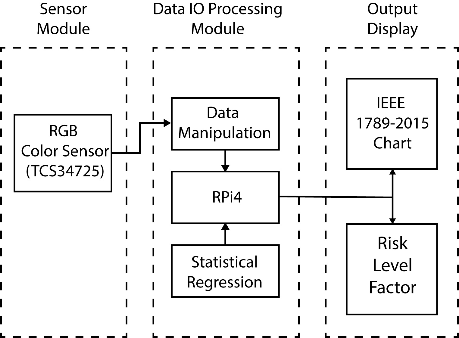
Fig. 5. Block diagram of modules for lighting control system.

Figure 6 depicts the flowchart of the measurement and simulation. In general, the lighting space’s lighting intensity variations are detected and measured by the sensor. Next, the data is used to generate and analyse waveforms. Hence, flicker performance is assessed by comparing it to industry standards. Finally, multiple statistical regression is used to evaluate the flicker level factor using the data from the waveform analysis.

Figure 6

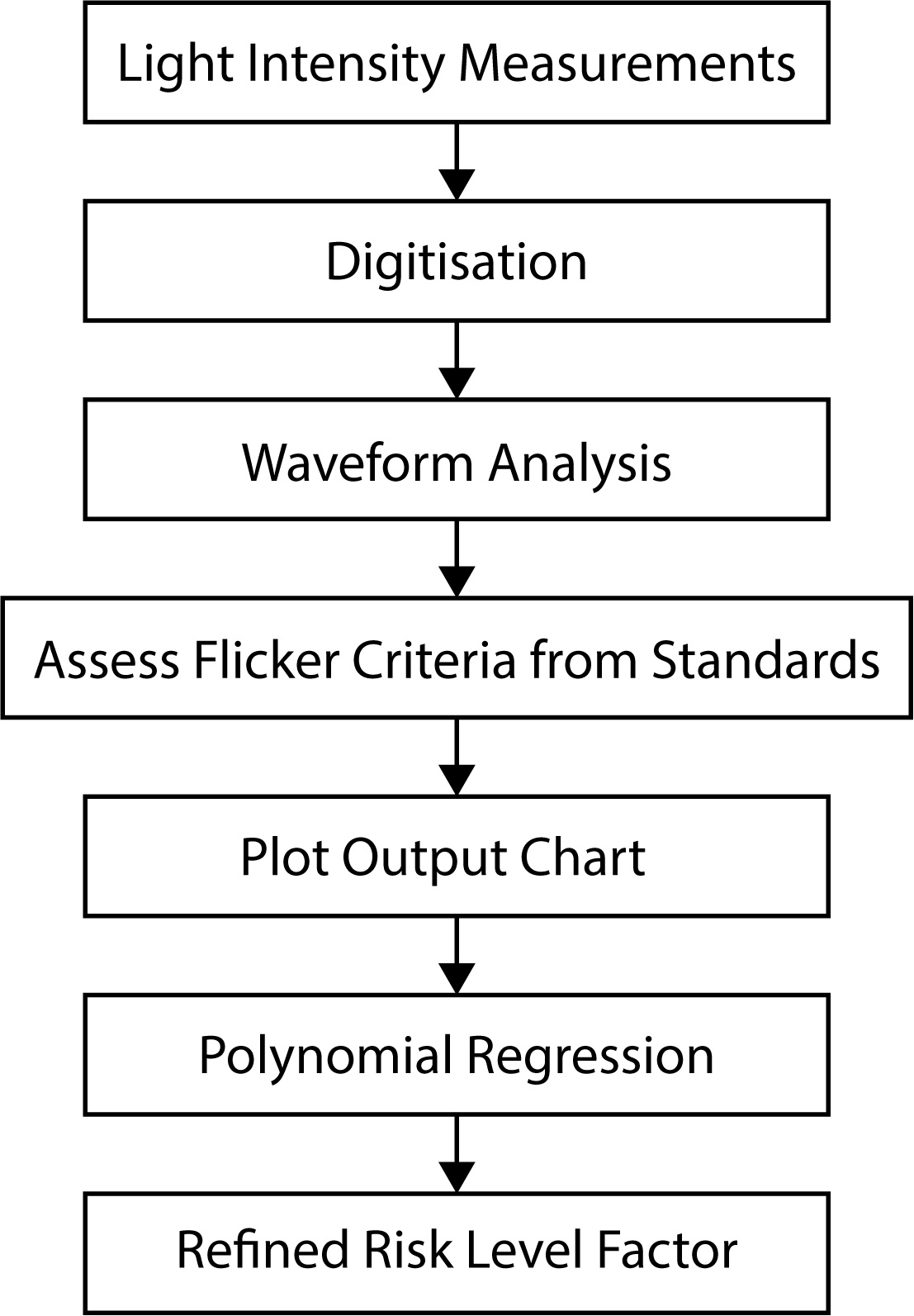
Fig. 6. Flowchart of lighting-space flicker risk determination.

3.1. TCS34725 sensor

In the electronics market today, various light sensors can detect lighting intensity fluctuations. They range from low-cost to high-cost. Sensors may be in standalone photodiode chips or an integrated circuit with a combination of Analogue to Digital converter (ADC) and photodiodes. One commonly available low-cost sensor unit with ADC built-in is the TCS43725 RGB colour sensor [19]. The support from the online community in providing application notes and driver libraries are abundant. As compared to illuminance or colour sensors, direct luminance sensors are more expensive. A high-performance luminance metre will cost over USD 300 in the electronics industry, while a TCS34725 sensor costs around USD 3.00 [9]. Albeit its low-cost, the sensor has been used successfully in robotic and other colour detection applications and researches [20,21].

3.1.1. Characteristics

Table 5 tabulates the characteristics of the TCS34725 RGB colour sensor. The sensor could read the intensity of lighting via photodiodes on four different channels. In addition, it has an integrated ADC that converts lighting intensity to digital values [19,22,23].

Also, lighting space illuminances (lx) and correlated colour temperatures (CCT) can be calculated using data from each channel. The sensor has a 400 kHz clock frequency. The clock frequency is an important consideration when choosing a sensor because low clock frequencies cannot sample high-frequency flickers.

Table 5

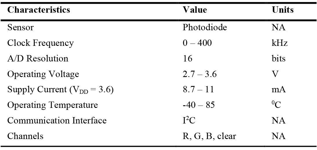
Table 5. Risk classification of WELL L07 Part 2.

3.1.2. Sensor application

Data from one channel is deemed sufficient for lighting flicker measurements. Therefore, the “clear” channel is chosen for the system. Figure 7 shows the red, green, and blue channels’ strength summation values. Other channels are filtered to output intensities on dominant wavelengths for red, green, and blue in the lighting spectrum. They are not used because they could distort lighting conditions that use a variety of CCTs. Therefore, the clear channel data represent the spectrum additions of red, green and blue components and are more suited for luminance and illuminance measurements, similar to human’s perception of visible lighting.

Figure 7

Fig. 7. Photodiode spectral responsivity [19].

Lighting intensity data are stored at memory registers in the ranges of 0 to 65, 535 (16 bits – 2 bytes). Only the lower, 8-bit (256-decimal) byte is of interest. Moreover, the memory address for the clear channel is 0x14 (hex format). The measurement system uses a sensor driver library provided by Dexter Industries [23]. The codings are written in Python language. The driver library allows the minicomputer to access and control the sensor (RPi4). Figure 8 depicts the flow for sensor initialisation, data retrieval, and offline storage. The loop in the flow will keep measuring and recording data for 2 seconds. In the actual built environment, the loop can be set to run every alternate minute to send flicker rating reports to building owners. For the testing purpose in this research, they are run on demand.

Figure 8

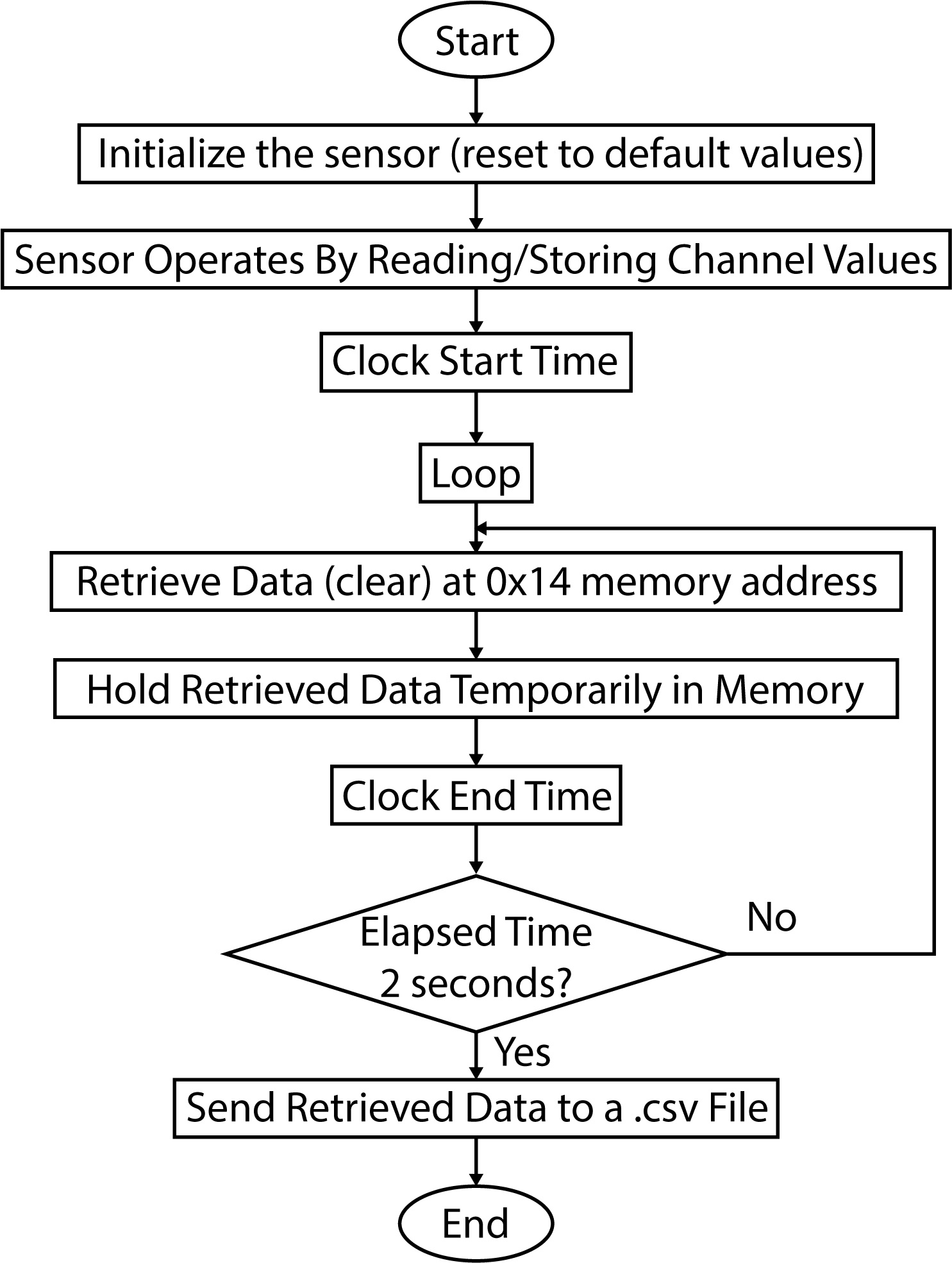
Fig. 8. Sensor operation flow.

The temporary data stored in the memory array is sent to a comma-separated value (CSV) file once the loop in Fig. 8 is completed. Waveforms are processed and generated using data from the CSV file.

3.2. Measurements & data processing

3.2.1. Raspberry Pi 4 minicomputer

An RPi4 minicomputer is chosen because of its size versatility. It is about the size of a credit card and can go anywhere in a lighting room. The Raspbian operating system runs on the RPi4 minicomputer. The normalised intensity values collected from the sensor are then stored in a memory of RPi4. Finally, they are processed and analysed for further action.

The RPi4 has Digital Input/Output pins that could receive signals from third-party sensors such as the TCS34725 [24-26]. RPi4 and TCS34725 sensors communicate through the I2C protocol. I2C is a bit-by-bit serial communication interface that sends and receives data [25]. A large amount of data can take longer to transfer between the host (RPi4) and the client (sensor). Therefore, careful consideration is taken by coding optimally to retrieve data from the sensor. Inefficient data retrieval coding may cause the read/write period to be delayed, affecting the sampling time. Figure 9 shows the schematic diagram of the RPi4 connected to the sensor, whereas Fig. 10 shows the breadboard level connections of both units.

Figure 9

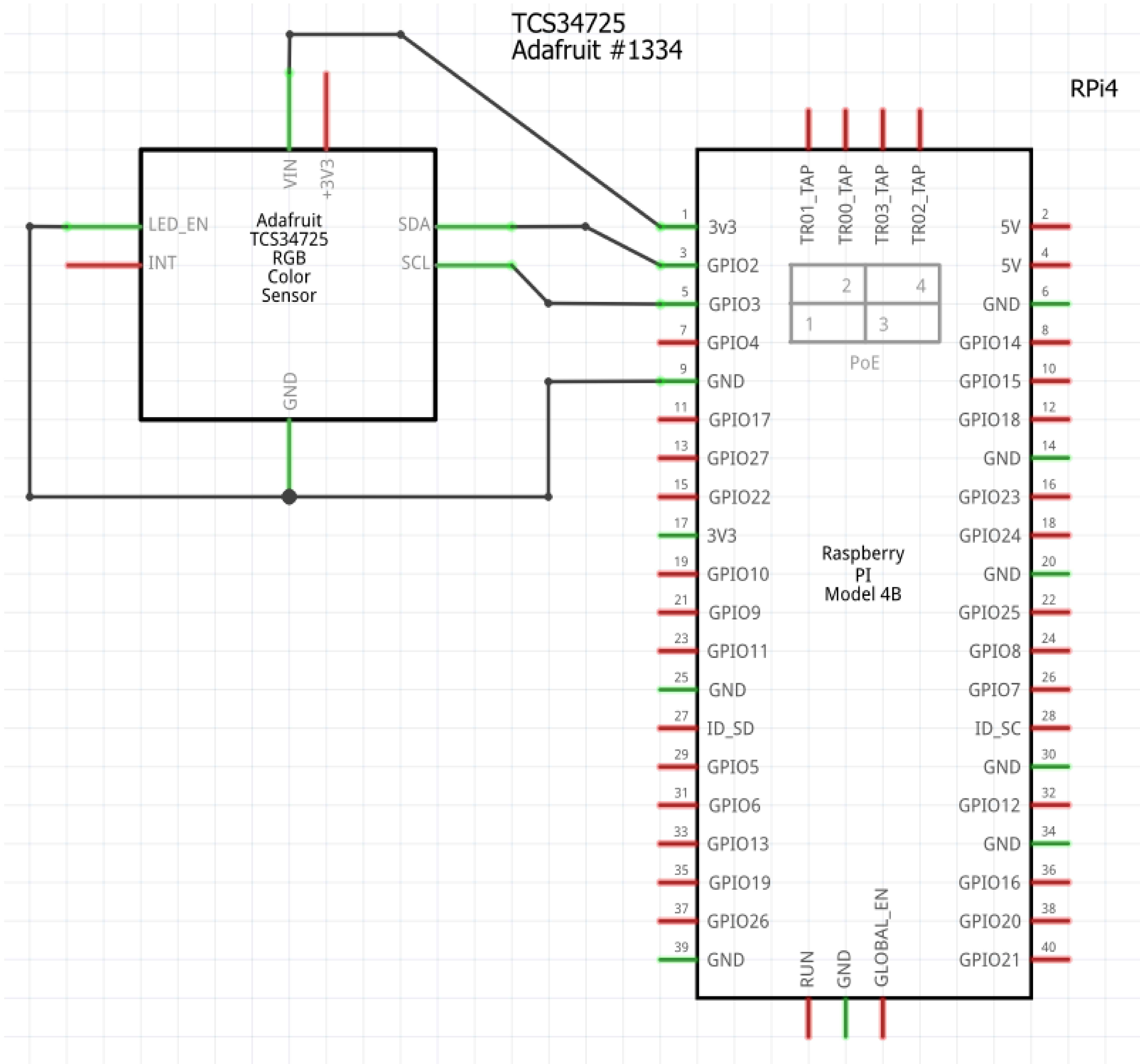
Fig. 9. Schematic diagram of RPi4 and TCS34725.

Figure 10

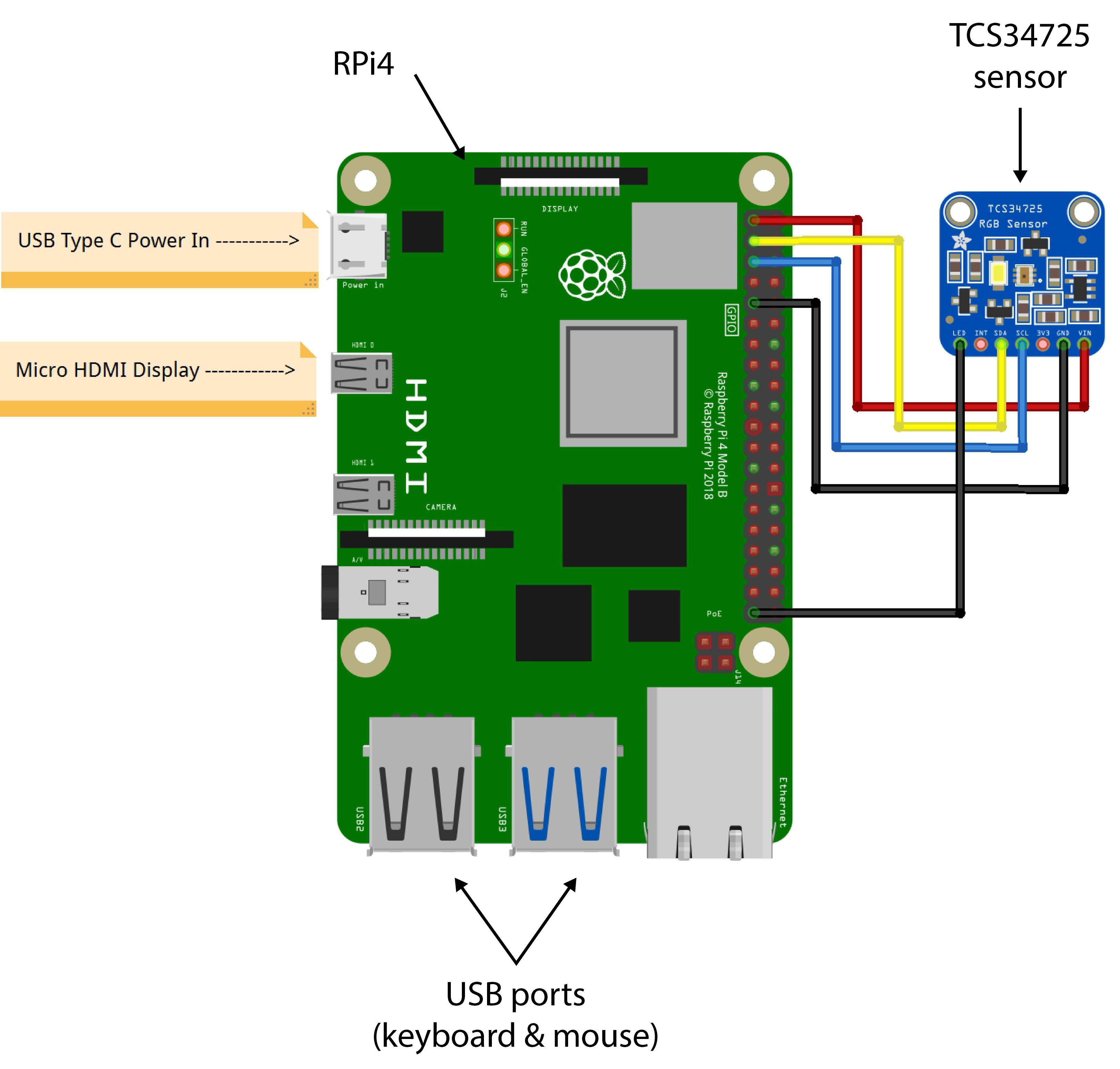
Fig. 10. Breadboard level connections of RPi4 and TCS34725.

3.2.2. Measurement procedure

There are a variety of lighting devices with various properties in any lighting room. For example, a bulb can have a high lumen output as compared to others. In addition, the CCT ratings of different bulbs can differ too. Therefore, this article focuses on measuring the average lighting intensity of a room through the sensor’s clear channel photodiode, Fig. 7.

Two units of 6-inch circular LED lighting have been installed in the room. They are each rated 15 watts at 3000 K CCT. Their operating voltages range from 220 to 240 volts, and their maximum lumen output is 1200 lm at 50 Hz. An electronic driver is included with each LED fixture.

Figure 11 depicts the room layout and the LED lighting placements. The room has a large window and a door. The existence of windows or doors does not matter as the measurement detects ambient lighting fluctuations in the room. The room’s ambient lighting intensity is a mixture of lighting from artificial lighting and natural daylighting during morning hours. If there are flickers from the LED lighting, it would still show in the lighting waveform through intensity changes. The ambient lighting flicker rating is determined by waveform analysis later through the percent flicker or flicker index. However, if severe flicker exists during measurements and analysis, it would have to be root-caused by building owners. For example, it may be due to external lighting being introduced to the room through the open door. Occurrences such as this pave the opportunity for building owners to take corrective action when flicker non-conformance are reported.

Figure 11

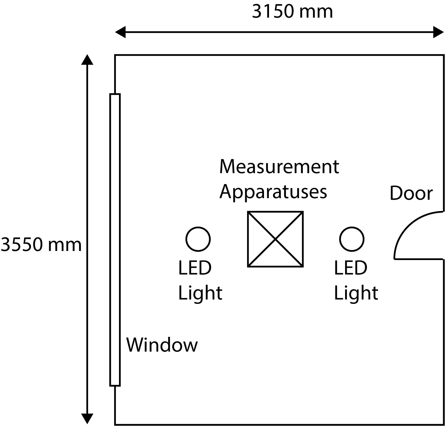
Fig. 11. Room layout.

As daylight lighting intensity fluctuations are null when there are no external stroboscopic influences, the measurement for this research was done during nighttime. It is to be noted that ceiling fans or other moving objects that obstruct lighting sources may cause flickers. However, the proposed flicker detection system is robust in that it will detect flicker caused by moving objects obstructing the lighting source. Nighttime measurements give more focus to the LED lighting installed. For this experiment, the measuring equipment is positioned in the middle of the room.

When all is in place, the sensor measures the room’s lighting intensity fluctuations and stores the information in the minicomputer. A time-series light source waveform is formed by taking continuous measurements for 2 seconds. It is possible to populate data for longer than 2 seconds, but this may add more noise. If much noise is present, determining the frequency of the waveform would be difficult.

3.2.3. Luminance and relative intensity

In most rooms, the different surfaces have different colours and material properties. As a result, these surfaces can reflect varying amounts of lighting, altering the lighting distribution in the room. The reflectance index of lighting space affects the brightness (luminance) of a lighting space [8,27]. Reflectance index is mathematically the ratio of reflected lighting to incident light. On the other hand, illuminance is the measure of lighting falling onto a surface area. The illuminance on wall surfaces or tabletops is an example of luminances reflected in objects. For a fully diffusely-reflecting surface (Lambertian surface), illuminance and luminance are linked, as shown in Eq. 4 below [28,29]. In contrast, typical lighting spaces need the reflectance index to balance the equation due to the existence of non-Lambertian surfaces – Eq. (5).

\[ E=L\pi \]

\[ E\rho=L\pi \]

where E is the illuminance (lux), L is the luminance (lumens), ρ is the reflectance coefficient/index, and π is the mathematical constant pi (~3.142).

For flicker measurements of discrete light sources, luminance is the accurate parameter when determining flicker modulation instead of illuminance [7]. This research uses illuminance as the source for flicker ratings due to two reasons. First, in a lighting space, the perceived brightness for occupants is illuminance. The luminance value decreases at a distance away from the light source (inverse distance square law). Secondly, differences in the sensor’s channel data (photodiode voltage fluctuations) are directly proportional to lighting intensity and luminance changes. The sensor channel’s 8-bit data parameter is equal in magnitude and variance for flicker measurements since the room’s reflectance index and pi are constants as in Eq. 5. Thus, this research assumes that the absolute magnitude of luminance is equivalent to illuminance. Therefore, luminance is not measured but assumed to be equivalent to illuminance. Hence, it could be normalised between 0 to 1 and used accordingly for flicker calculations. The same is true for changes in voltages or currents caused by a shift in the lighting waveform amplitude. In LED lighting technology, the LED driver can be either a constant voltage (c.v) or current (c.c) type. As such, Eq. 6 applies to LED lighting drivers of AC or DC drivers in tandem with the assumption [4,7].

\[ ∆E α ∆A α ∆Vcc α ∆Icc \]

where ∆E is the changes in illuminance, ∆a is the changes in lighting waveform amplitudes, ∆V_cc is the changes in the sensor’s photodiode voltages (constant-current drivers), and ∆I_cc is the changes in the sensor’s photodiode currents (constant-voltage drivers).

3.3. Waveform generation & standard compliance check

The RPi4’s memory storage is accessed to retrieve digital data measurements corresponding to light intensity. They are referred to as “word” (16-bit) rather than “byte” (8-bit). A lighting waveform is generated using the 16-bit data. The amplitude variance is plotted from minimum to maximum values. To reflect the extracted values as relative light intensity, they are first normalised between 0 (0 decimal) and 1 (255 decimal). Hence, a time-domain relative lighting intensity waveform is generated.

All data processing and analysis use the Python scripting tool. Python has a large number of open-source libraries with data crunching and calculation features. The libraries used in this article are mainly from Python’s ecosystem, specifically, NumPy and SciPy, which support mathematical and signal processing work, respectively [30,31]. In addition, Python’s Matplotlib library is used to build graphical plots [32].

3.3.1. Sampling time

The sampling time must be determined before the waveforms can be produced. The time for each successive measurement is referred to as sampling time. For RPi4, the measurement interval is not constant due to the RPi4 and sensor electronic circuitry’s intrinsic noises. Sampling time is determined by taking the average time differences between each reading from the memory register for the clear channel. Table 6 tabulates an example of the case. The mean value is the sampling time.

Table 6

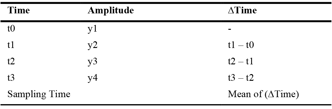
Table 6. Determination of sampling time.

3.3.2. Signal noise filtration

Noises from the waveform should be removed to achieve a smoother waveform shape. A Savitzky-Golay filtering technique is used to achieve this (Fig. 12) [30]. A Savitzky–Golay filter smooths the data by applying a digital filter to a series of data points. It also improves data accuracy without distorting the signal’s properties. Curve smoothing is accomplished by mathematical function convolution. It involves fitting successive subsets of adjacent data points with a low-degree polynomial using the linear least-squares method. Python’s SciPy library has a tool to automate this procedure.

Figure 12

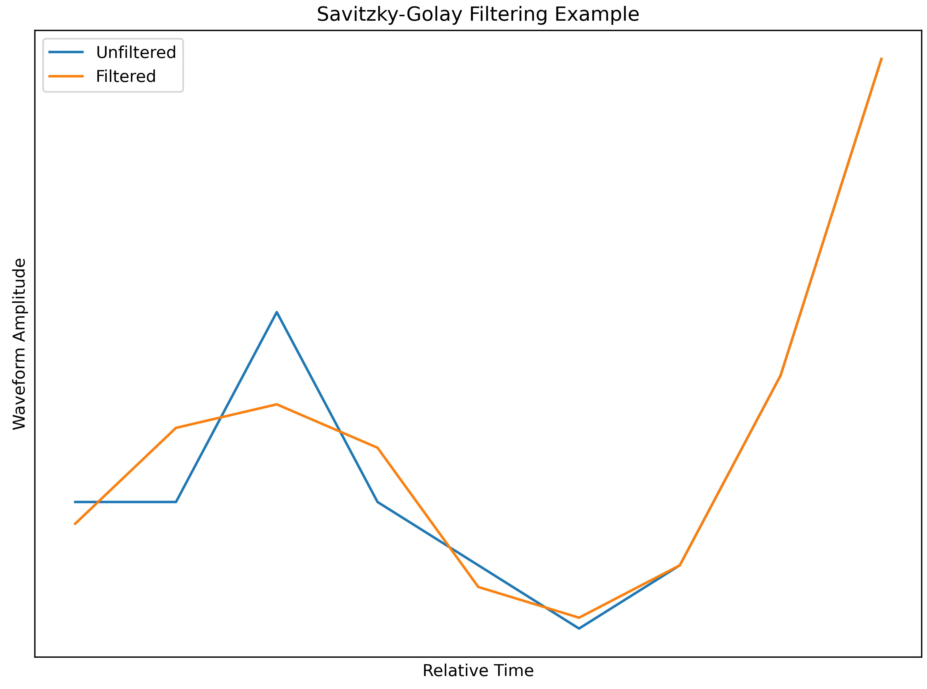
Fig. 12. Savitzky-Golay filtering to remove noise.

3.3.3. Signal frequency

The waveform frequency is one of the most critical parameters to determine. Waveform frequency is found using Zero-Crossing Method (ZCM). The frequency estimation via ZCM is ensured to be accurate with the Fourier Fast Transform (FFT) method [30].

The ZCM is a method for detecting the locations of amplitudes along the zero-axis by scanning them consecutively. What matters is whether they are above or below the zero-axis. The zero-axis is normalised to the average values of all amplitudes before that. The number of points above and below the zero-axis is evaluated by comparing the amplitude sign changes. A relative time interval between consecutive amplitudes can be calculated by taking the mean of the sum of points above and below the zero-axis and dividing by a constant factor of two – Nyquist Frequency Theorem. The theorem states that the sampling rate must be at least twice the waveform’s maximum frequency; thus, the constant factor two, to digitise a waveform without aliasing. Finally, multiplying the sampling rate by the relative time interval scales the relative time interval to the actual frequency.

FFT is a method similar to ZCM to determine the waveform frequency. Typical lighting space flicker waveform constitutes many frequencies, such as noises. FFT transforms the time-domain signal to a frequency-domain signal and populates all the frequency contents of the signal using Fourier analysis. The relative intensity of each frequency content is known from FFT and can be plotted in a graph. The most dominant frequency with the highest intensity usually represents the nominal propagating frequency of the waveform.

3.3.4. Flicker from signal

The following formulas calculate the percent flicker and flicker index from the waveform generated [31,33].

\[ V_{pp}=\ V_{max}-V_{min} \]

\[ PF=\ \left(\frac{V_{pp}}{V_{max}+V_{min}}\right)\times100\ % \]

where V_pp is the peak-to-peak voltage of the waveform, V_min is the minimum voltage of the waveform, V_max is the maximum voltage of the waveform, and PF is the percent flicker (%).

Furthermore, because the measurements obtained by the sensor are voltage correlated, the Voltage (V) sign can be interchanged with Luminance (L), Illuminance (E), or Amplitude (A).

The waveform is divided into the top half and bottom half around the average value to evaluate the flicker index, similar to Fig. 2. The statistical mean of the amplitude values from the data points is the average value. The area is then calculated by integrating the top and bottom halves’ data points through the time interval. The integration technique is used to calculate the waveform area that covers the top and bottom half. These steps are only applied to one cycle.

\[ FI=\ \left(\frac{A_{top}}{A_{top}+A_{bottom}}\right) \]

where FI is the flicker Index, A_top is the area of the top half of the waveform above the average value, and A_bottom is the area of the bottom half of the waveform below the average value

The flicker percent and index are used to assess the standard compliance based on the criteria from Tables 2, 3 and 4.

3.4 Refining the low-risk region of ieee 1789-2015 chart

Figure 13 displays a continuum of min and max modulation values for all frequencies in the low-risk region shaded yellow. A correlation is applied to determine the precise risk level factor ranging from 0 to 1 using the min and max values through polynomial regressions [30]. The highest (1) risk level is near the top zone, shaded red, and lowest (0) near the bottom zone, shaded green. Waveforms that fall into the green or red zones are categorised as “no risk” or “high risk,” respectively. Further correlations may be drawn between the red and green areas, but they are insignificant for this paper. Flicker-free lighting must be maintained in all facilities. If, on the other hand, the output falls into the red zone, an urgent corrective action plan with emergency funds must be implemented to eliminate the health risks associated with lighting flickers.

Figure 13

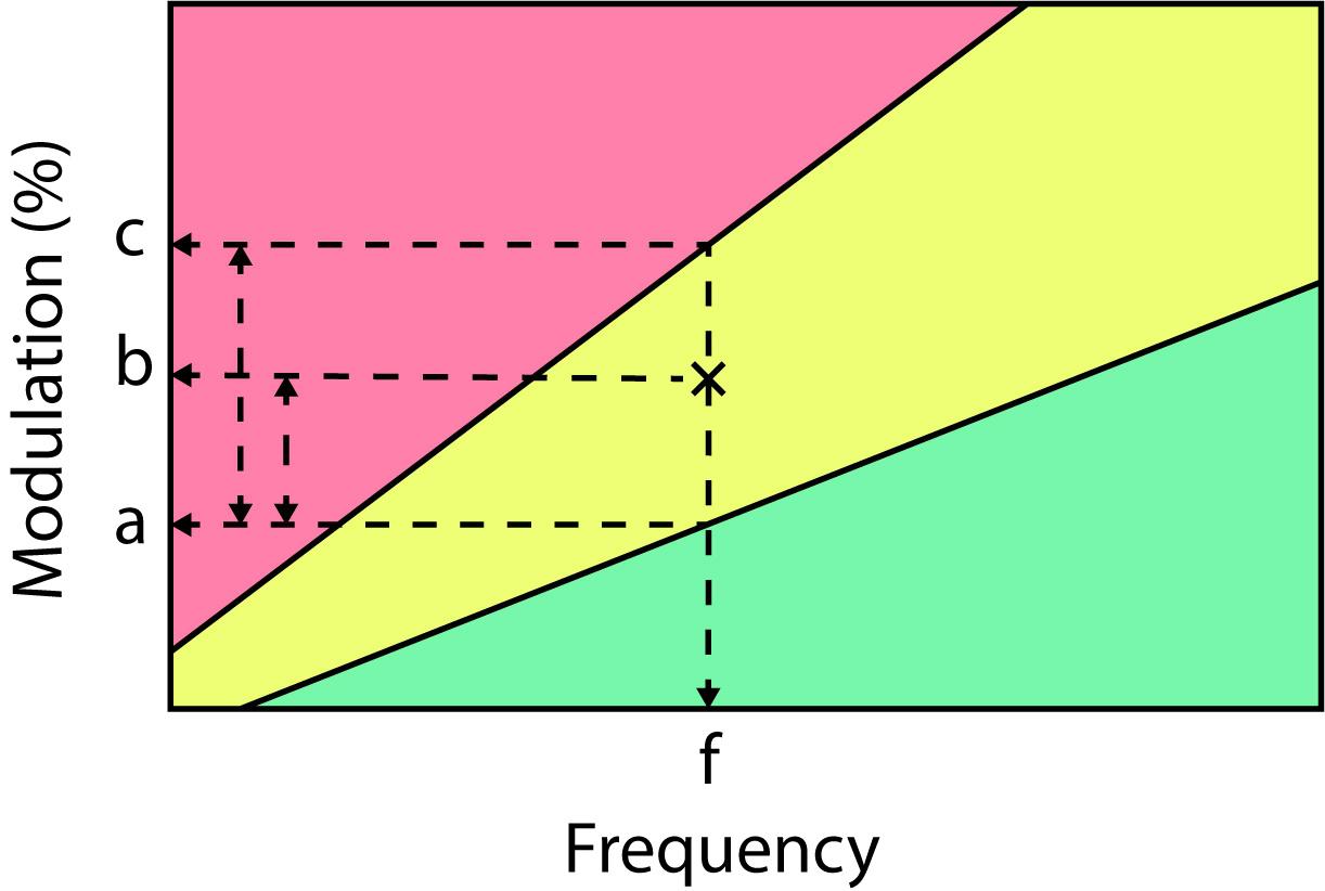
Fig. 13. Maximum and minimum correlation.

Therefore, the normalisation between 0 and 1 for the yellow zone in Fig. 13 is determined. The 0 and 1 normalisation output numbers can be adjusted to accommodate various facility risk-assessment rating levels.

\[ \frac{b-a}{c-a}=\ \frac{x-0}{1-0}\Longrightarrow\ x=\frac{b-a}{c-a} \]

where a is the Percent flicker (or modulation) at the intersection between dominant/operating frequency, f and borderline of low-risk (yellow zone) and no-risk (green zone), b is the calculated percent flicker (or modulation) for lighting space with dominant frequency, f, c is the percent flicker (or modulation) at the intersection between dominant/operating frequency, f and borderline of low-risk (yellow zone) and high-risk (red zone), and x is the refined flicker risk factor (in the marginal yellow zone).

4. Results and analysis

4.1. Hardware

Figures 14 and 15 shows the pictures of the measurement apparatus built. They are placed in the middle of the empty room, as described in Fig. 11.

Figure 14

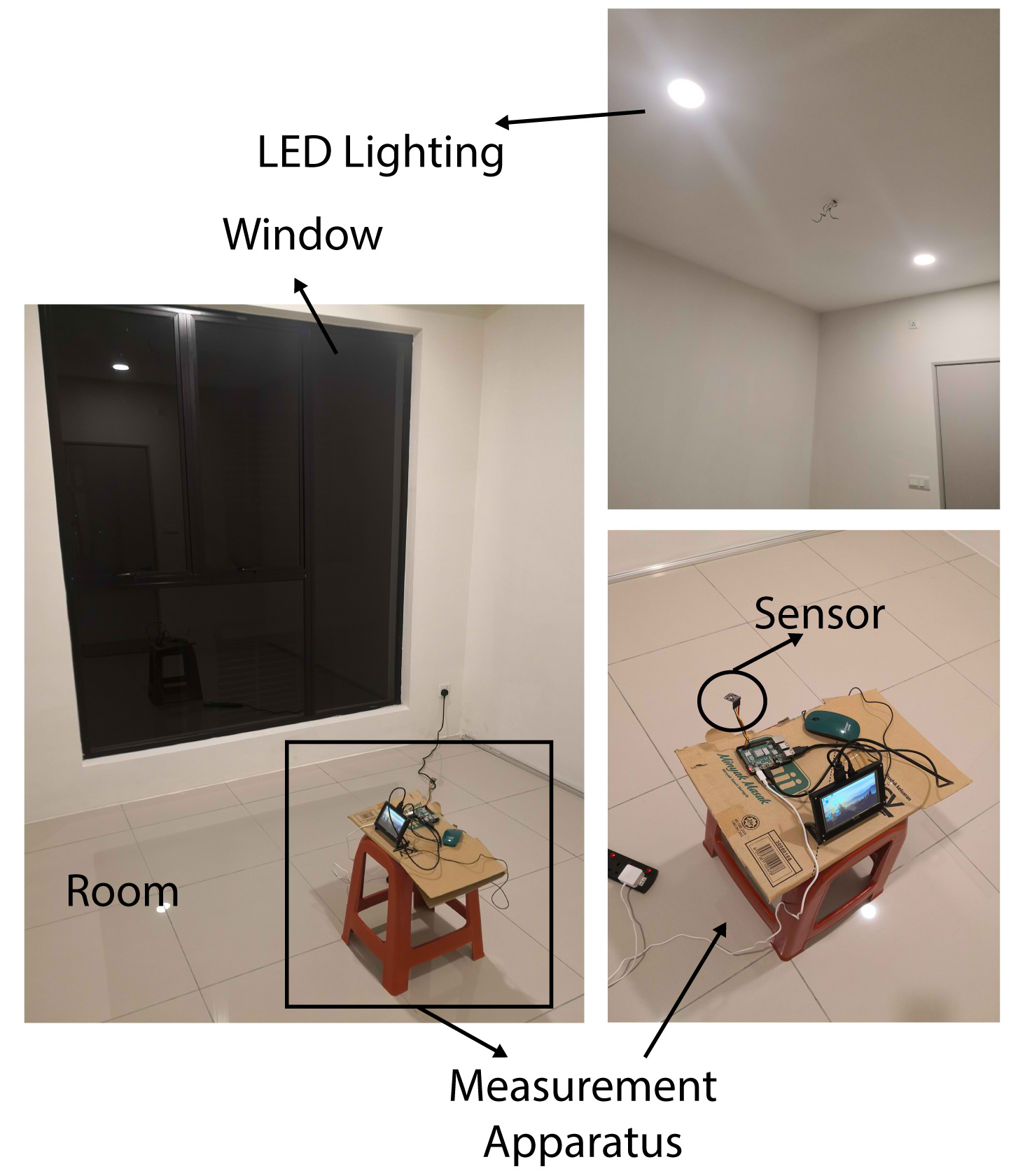
Fig. 14. Room setup & measurement apparatus.

Figure 15

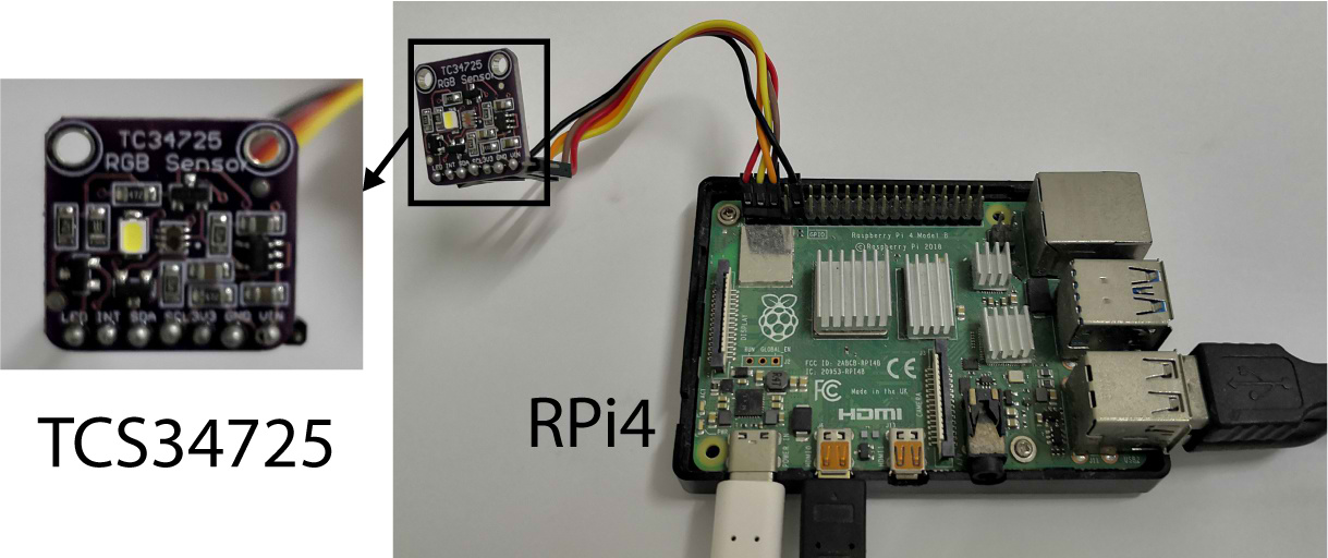
Fig. 15. Raspberry Pi4 minicomputer & TCS34725 colour sensor.

4.2. Measurements

Table 7 tabulates the first and last five data extracted from the CSV file. The sampling time is estimated to be about 0.000514 seconds based on the time value in row number 2. The time interval corresponds to a frequency of 1945 Hz. However, from column “Time” in Table 7, the sampling time for each measurement is not constant. Therefore, Table 6 is used to calculate an average value of 2014 Hz (0.0004965 seconds). The sampling time is determined by the sensor’s and minicomputer’s efficiency, and it is affected by a variety of factors such as temperature, CPU degradation, and others.

Table 7

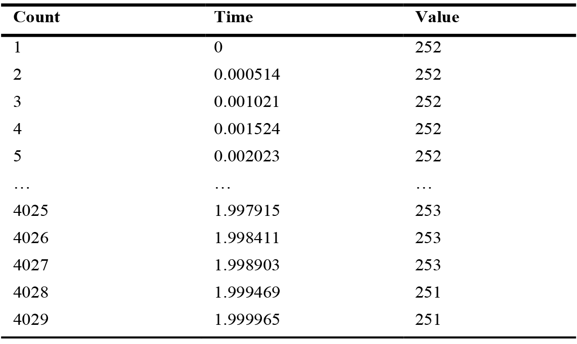
Table 7. Raw data measurements.

In Table 7, the column “Value” has values in the range of 0 to 255 (digitised values). Specifically, they are the 8-bit data encoded during the analogue-to-digital conversion phase at the sensor. In other words, they represent the instantaneous lighting intensity. By observing the readings, it can be noticed that the lighting produces only small intensity differences. Meaning, the lighting waveform is relatively smooth.

4.3. Waveform outcome

Figure 16 (with noise unfiltered) and Fig. 17 (denoised) show the waveform for the lighting in the room. For digitised values, denoising the raw waveform is not recommended since the percent flicker increases by 0.3 percent, making the waveform more harmful when plotted in the IEEE 1789-2015 chart. Therefore, the unfiltered waveform is used in the subsequent steps.

Figure 16

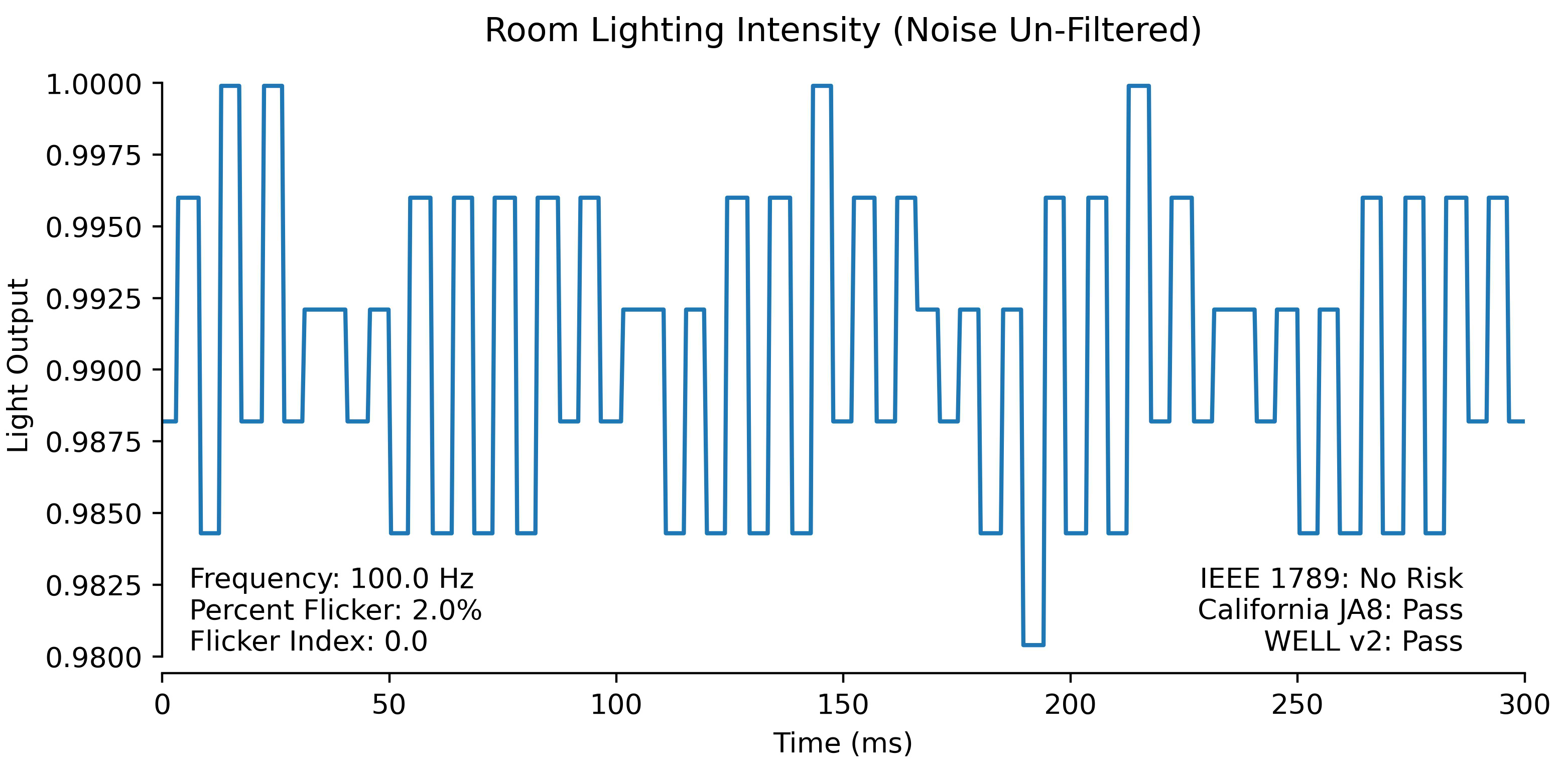
Fig. 16. Room flicker waveform unfiltered for noise.

Figure 17

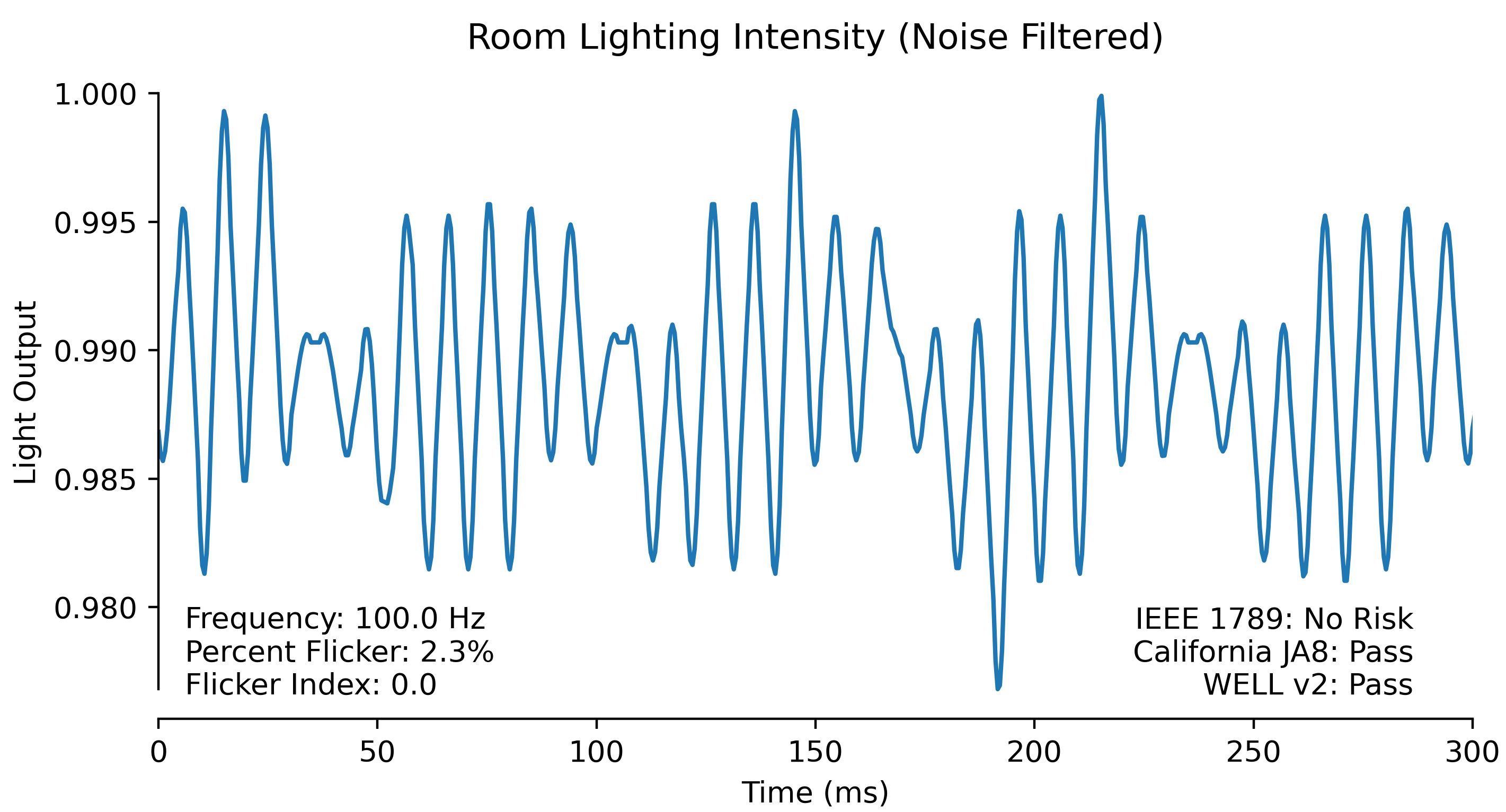
Fig. 17. Room flicker waveform (denoised).

Figure 16 shows the summary of the waveform in the lower-left corner. The zero-crossing method yields a frequency of about 99 Hz for the waveform. This value is consistent with the characteristics of a 50 Hz mains supply, in which flickers are typically seen at twice the main frequency. Percent flicker is calculated to be 2.0%. The flicker index is very low and has been rounded to zero. At the lower right corner of Fig. 16, the pass-fail criteria for the flicker standards are shown. The frequency of the waveform is confirmed to be 100 Hz when the FFT method is used. Whereby the result of the most dominant frequency for the waveform is determined as 99.96 Hz. Figure 18 shows the frequency domain analysis of the waveform.

Figure 18

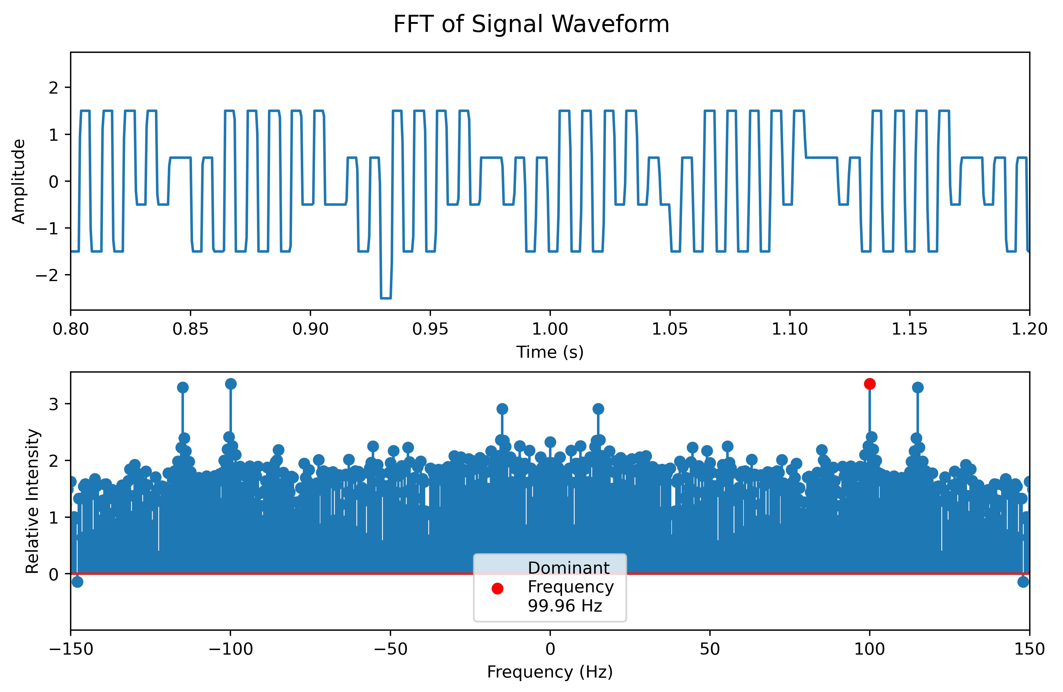
Fig. 18. FFT of room lighting waveform.

In a nutshell, the room lighting waveform meets all three standard requirements summarised in the plot’s lower-right text in Figs. 16 or 17. In cases of flicker rating which fails a specific standard, more so to IEEE 1789-2015 criteria, it is suggested that the building owners take corrective action plans to rectify the flicker issues in the lighting space. Corrective actions range from changing luminaries in the room to safer (safety certified) ones to vacating occupants from the room. These actions go back to building management teams and safety teams to assess and devise a strategy with management teams. In cases of needs to put forward proposals to finance or management teams, the results such as above may be used to substantiate budget requests for retrofitting lamps. In a later section, through refined risk level determination results, a precise figure can further validate the budget requests when flicker ratings are marginal.

4.4. IEEE 1789-2015 Chart

Figure 19 shows the room flicker rating values of 99 Hz at 2.0 percent flicker (modulation) plotted on the IEEE 1789-2015 chart. It is worth noting that the point’s location is on the dividing line between low-risk and no-risk zones. This occurrence presents an opportunity to further fine-tuning the risk rating to decimal values.

Figure 19

Fig. 19. IEEE 1789-2015 flicker risk zones for room lighting.

4.5. Refined risk level output

Table 8 and Fig. 20 shows how the borderline between high-risk and low-risk (top border) is interpolated using regression to derive a polynomial function. Similarly, Fig. 21 shows the graphs for the bottom border.

Table 8

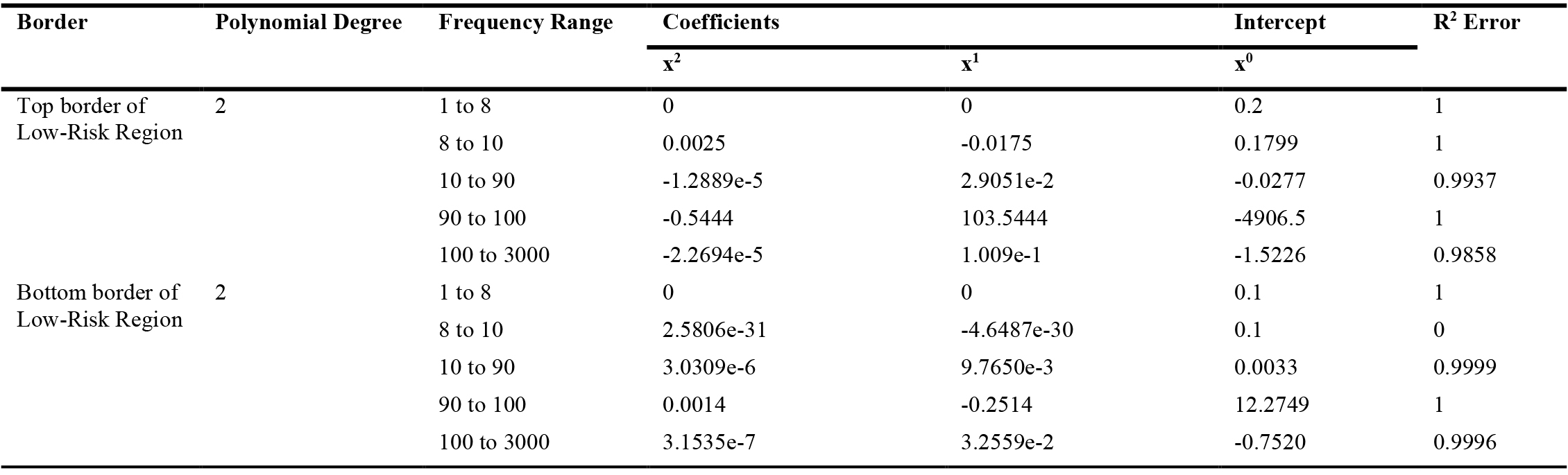
Table 8. Regression parameters for border lines.

Figure 20

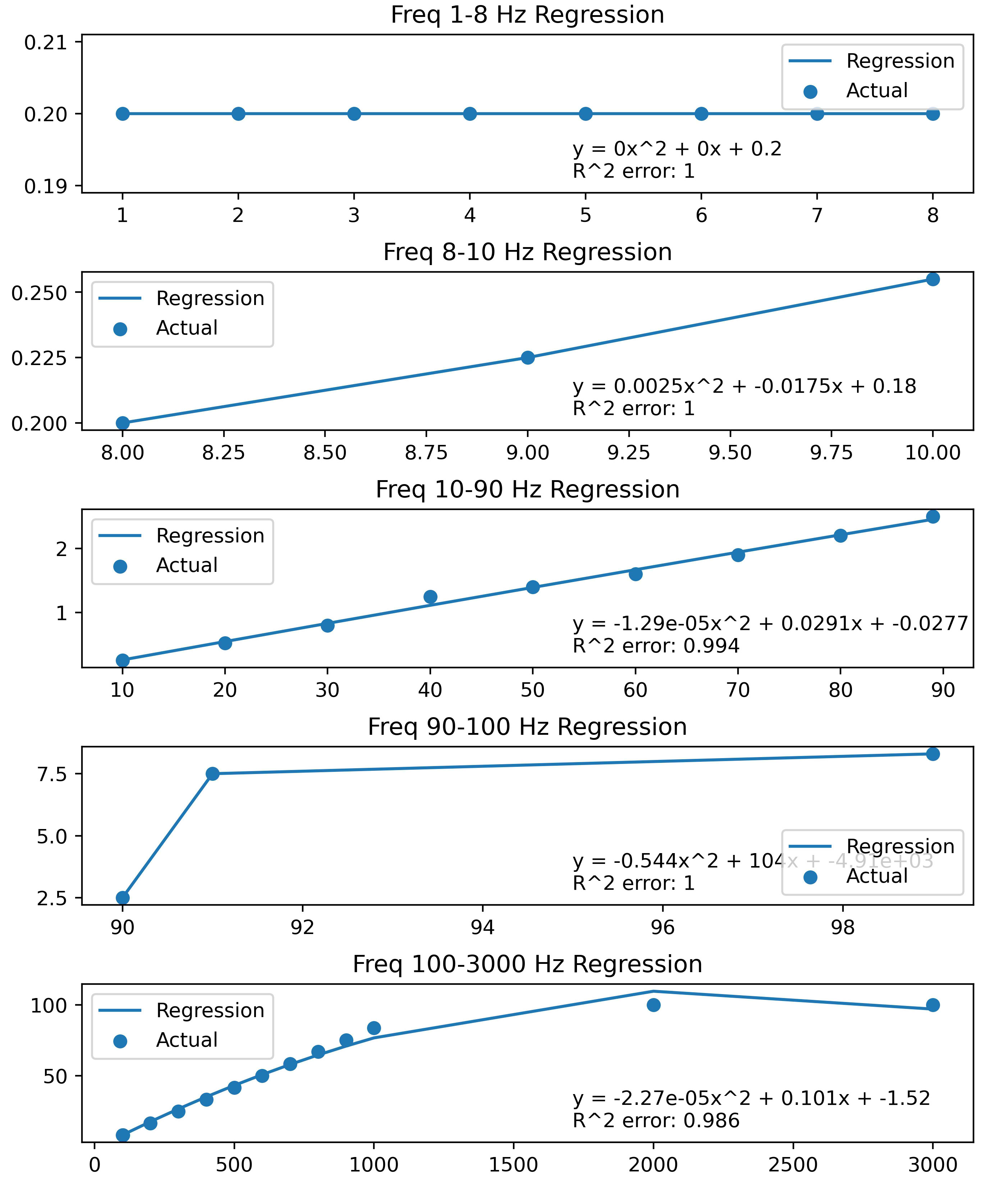
Fig. 20. Regression of top border of low-risk zone.

Figure 21

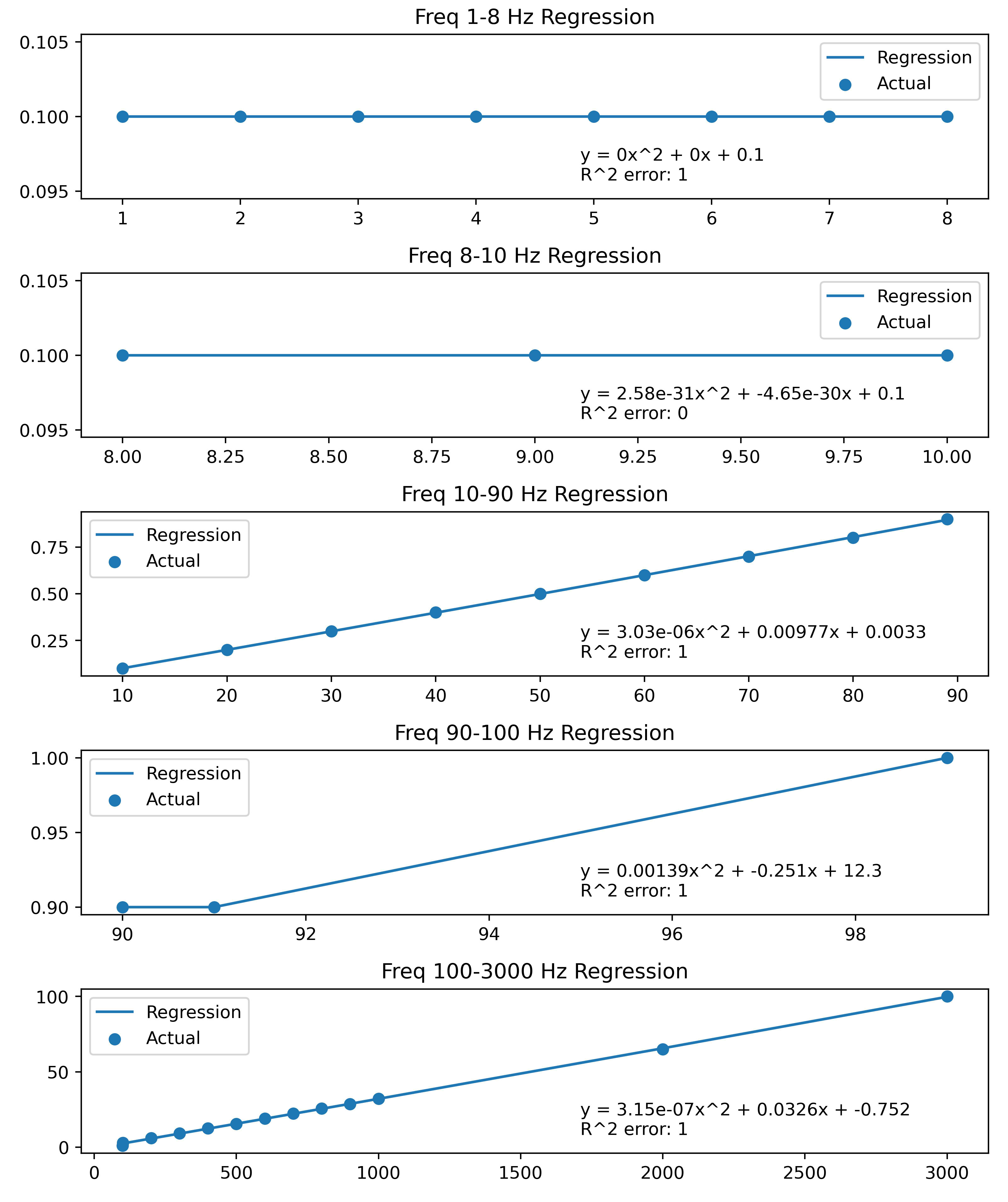
Fig. 21. Regression of bottom border of low-risk zone.

Therefore, the refined risk level factor for the room lighting, which was at 99 Hz, is determined using Eq. 10. Table 9 presents the outcome.

Table 9

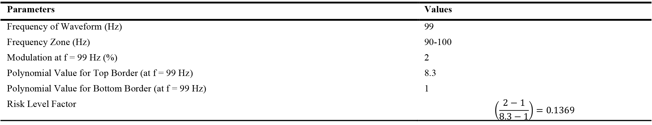
Table 9. Regression parameters for border lines.

When looking at the point “room” in Fig. 19, the point appears to be in the middle of the yellow zone (low-risk region). However, the risk level factor is less than half because the chart is on a logarithmic scale.

4.6. Application of refined risk level factor as likelihood in risk assessment

The refined risk level factor may be used in many scenarios. As mentioned in Section: Refined Flicker Risk Level, one of the uses of the factor is to substantiate a budgetary request for corrective action plans. A test simulation using the refined risk level factor in a risk matrix assessment is presented in this section.

After measuring the flicker ratings and calculating the refined risk level factor in a built environment, the refined risk level factor is used as a likelihood variable in a risk assessment matrix, as shown in Table 10.

Table 10

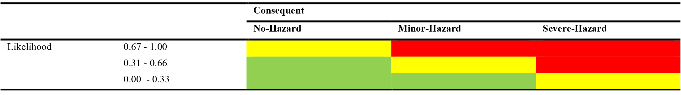
Table 10. Sample risk matrix for test simulation.

In Table 10, the red, yellow and green coloured cells represent high, low and no-risk levels.

The consequent (flicker effects on humans) of hazards are tabulated in Table 11 as follows (adapted from [4]).

Table 11

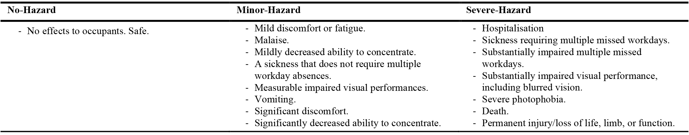
Table 11. Hazard classification for test risk matrix simulation.

From the case of the “room” point in Fig. 19, the refined risk level, which was calculated to be 0.1369, falls in the lowest category of defined likehoods as per Table 10. Matching to symptoms that could occur to occupants in a building as per Table 11, the risk level can be pinpointed, followed by corrective action plans if needed. For example, if an occupant complains of having vomiting symptoms, the room lighting level is deemed low-risk. Although low-risk may sound not so severe for vomiting cases, the flicker rating is still within the acceptable range for lighting flicker assessments. There may be other non-lighting factors that need to be root-caused by building owners in particular facility and safety teams. However, on the same note, facility teams can start replacing lamps in the room due to the low-risk rating in phases by requesting replacement budgets to management teams. The refined risk level factor aids in putting forward a monetary figure as substantiation for replacement works. Table 12 summarises an example of a budget request.

Table 12

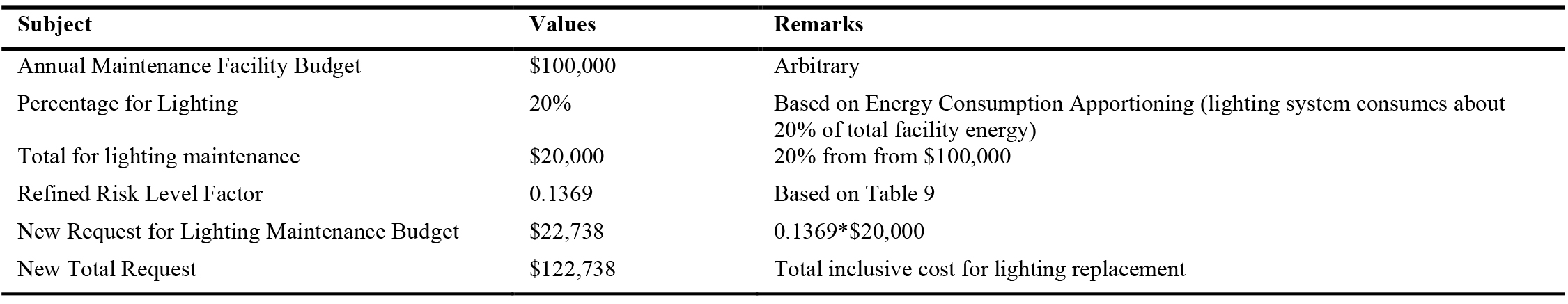
Table 12. Budget request to include lighting replacement works in phases.

However, for high-risk ratings, immediate urgent corrective action plans should be taken. When risk ratings are none or no-risk, continuous monitoring is recommended.

5. Discussions

5.1. Sampling Time of TCS34725

There are a few sensor driver libraries available online, most notably from Adafruit Industries and Dexter Industries. The function to access the sensor memory for digital data of lighting intensity from the drivers takes about 0.0025 seconds (500 Hz). The low-frequency value is because the function performs read/write operations through the I2C protocol four times to collect data for four channels and reads other memory registers. The channels are Red, Green, Blue, and Clear. For flicker measurements, only the “clear” channel data is required. The driver library coding is modified offline to access only the particular channel. After modification, the sampling time improves to 0.0004965 seconds (~2000 Hz). Having a higher sampling rate gives a more accurate rendering of the flicker waveform. A slower sampling rate may distort the generated waveform as it represents the actual signal less. Some peaks and troughs may be missed or not captured by a low sampling rate.

The library driver also has a delay of 2.4 ms between consecutive readings. This delay, referred to as integration time in the library, is introduced to omit redundant measurements. Increased sensitivity at low light levels can be achieved by using longer integration times. However, the room is not dark, and the delay is not needed for flicker measurement and thus removed. Flicker measurements need high-resolution sampling.

5.2. Sensor gain

The gain parameter is yet another sensor configuration. Gain amplifies the signal to a level where the A/D converter can accurately scale it. Higher gain settings amplify noises too. However, without gain, the sensor would be unable to differentiate those signals from ambient noise. The sensor has a 3.8 million-to-one dynamic range for A/D conversion resolution. Signals with small amplitude change would only utilise few bits in the conversion range. Therefore, amplifying the signal increases the precision of measured values.

5.3. Building monitoring system (BMS) /building automation system (BAS) and internet of things (IoT)

Facility maintenance teams monitor and control building engineering parameters through BMS, BAS, and the likes. Most of the monitoring system deals with building air-conditioning system, fire protection system, electrical power statutes, process parameters, and others. Sensors or actuators attached to the engineering system communicates between the host (main server) and client (engineering system) through different types of communication protocols such as BACnet (Building Automation and Control (BAC) networks). BACnet protocol operates on serial communication and data exchange through a local network. The flicker monitoring system is similar to the sensor and host (RPi4) communicate through the I2C protocol (serial communication). RPi4 has network connectivity capabilities. There are also home automation libraries and software that utilise RPi4 as a host. Similar to the industry-standard BACnet, residential application is possible. Therefore, by linking RPi4 to the BMS/BAS server, data could be exchanged. This article only focuses on the flicker measurement and simulation procedures.

With the advent of automation technologies and Internet accessibility, measurements and sensor data could be monitored remotely, where in some cases, actions could be taken. These are the concept of the Internet of Things (IoT), in which a flicker monitoring system could be integrated for occupant’s well-being.

6. Conclusions

In summary, this paper aimed to detect lighting space flickers. The concept of a lighting space flicker measurement and monitoring system was described in this article using a TCS34725 RGB colour sensor and an RPi4 minicomputer, which acts as a building automation server. The flicker measurement is achieved using the TCS34725 colour sensor to detect lighting intensity variations through its photodiodes. Changes in the photodiode readings were digitised through the sensor’s internal ADC. Further, a minicomputer (RPi4) is used for waveform generation and analysis. The outcome of the system is a risk level analysis of lighting flickers. Output is in graphical form, whereupon analysis, a room test lighting was found to be complying with all three flicker standards, namely IEEE 1789-2015, JA8 and WELL standards. In addition, the room test light was found to be in the marginal low-risk zone of the IEEE 1789-2015 standard, which, when further refined through polynomial regressions, were able to produce a precise risk level factor. The precise risk level factor may be used in budgetary needs or used as a likelihood variable in typical risk matrices. The system can be integrated into smart building lighting applications, where building owners can be alerted during non-conformance of flicker parameters.

Acknowledgment

The authors would like to state their gratitude to the Malaysian Ministry of Health and University Sains Malaysia for providing research funding, data, equipment, and support to publish this article.

Contributions

S. R. Perumal suggested the concept, tested it, gathered data, and oversaw the article’s writing. F. Baharum supervised the experiment and provided data analysis, debate, and assistance in cross-checking perspectives to develop this article.

Declaration of competing interest

This paper did not disclose any private, personal, and confidential data of anyone or organisations. The images are self-developed for educational purposes only by the authors or from the stated sources (if any).

References

L. L. A. Price, M. Khazova, and J. B. O’Hagan, Human responses to lighting based on LED lighting solutions, CIBSE-Public Health of United Kingdom Report, United Kingdom, 2016.
P. Boyce, Human Factors in Lighting, 2nd Edition, Taylor & Francis, London, 2003. https://doi.org/10.1201/9780203426340
M. Rossi, Circadian Lighting Design in the LED Era, Springer International Publishing, Italy, 2019. https://doi.org/10.1007/978-3-030-11087-1
IEEE Power Electronics Society Standards Committee, IEEE Standard 1789-2015, IEEE Recommended Practices for Modulating Current in High-Brightness LEDs for Mitigating Health Risks to Viewers Sponsored by the Standards Committee, United States, 2015. https://doi.org/10.1109/ieeestd.2015.7118618
I. Chew, V. Kalavally, N. W. Oo, and J. Parkkinen, Design of an energy-saving controller for an intelligent LED lighting system, Energy & Building 120 (2016) 1–9. https://doi.org/10.1016/j.enbuild.2016.03.041
J. Bullough, K. Sweater Hickcox, T. Klein, and N. Narendran, Effects of flicker characteristics from solid-state lighting on detection, acceptability and comfort, Lighting Research & Technology 43 (2011) 337-348. https://doi.org/10.1177/1477153511401983
N. M. Miller, Flicker in Solid-State Lighting : Measurement Techniques, and Proposed Reporting and Application Criteria (2013).
S. Kitsinelis, G. Zissis, and L. Arexis, A study on the flicker of commercial lamps, Light and Engineering 20-3 (2012) 58-64.
H. Salama and F. Bendary, Light flicker Performance of Low power LED Units, in: 25th International Conference on Electricity Distribution, 2019, p 960 Spain. https://doi.org/10.34890/428
I. Azcarate, J. J. Gutierrez, P. Saiz, A. Lazkano, L. A. Leturiondo, and K. Redondo, Flicker characteristics of efficient lighting assessed by the IEC flickermeter, Electric Power Systems Research 107 (2014) 21-27. https://doi.org/10.1016/j.epsr.2013.09.005
The Illuminating Engineering Society of North America (IESNA) Light Sources Committee, IESNA TM-16-05 Technical Memorandum on Light Emitting Diode (LED) Sources and Systems, United States, 2005.
P. Iacomussi, M. Radis, G. Rossi, and L. Rossi, Visual Comfort with LED Lighting, Energy Procedia 78 (2015) 729-734. https://doi.org/10.1016/j.egypro.2015.11.082
The California Energy Commission, Appendix JA8 – Qualification Requirements for High Efficacy Light Sources, Title 24, Part 6, Build. Energy Efficient Standard 17-BSTD-02, no. 223245–9, United Stated, 2018.
WELL Building Institute Pbc, WELL Building Standard L07 Part2, 2018. https://v2.wellcertified.com/v/en/light/feature/7.
N. J. Duijm, Recommendations on the use and design of risk matrices, Safety Science 76 (2015) 21-31. https://doi.org/10.1016/j.ssci.2015.02.014
K. G. Lough, R. Stone, and I. Y. Tumer, Function Based Risk Assessment: Mapping Function to Likelihood, in: 17th International Conference on Design Theory and Methodology, 2005. https://doi.org/10.1115/detc2005-85053
C. Liu, W. Chen, Y. Hou, and L. Ma, A new risk probability calculation method for urban ecological risk assessment, Environmental Research Letters 15 (2020) 24016. https://doi.org/10.1088/1748-9326/ab6667
C. Guanquan and W. Jinhui, Study on probability distribution of fire scenarios in risk assessment to emergency evacuation, Reliability Engineering & System Safety 99 (2012) 24-32. https://doi.org/10.1016/j.ress.2011.10.014
TAOS Incorporated, Datasheet - TCS34725 - Color Light-to-Digital Converter with IR Filter, United States, 2012.
H. Surana, N. Agarwal, A. Udaykumar, and R. Darekar, Blackbox-Based Night Vision Camouflage Robot for Defence Applications, Advances in Intelligent Systems and Computing 810 (2018) 631-637. https://doi.org/10.1007/978-981-13-1513-8_64
Z. Zou, Y. Wang, and M. Zhou, Design and testing of an apple grading control system, in: 2017 IEEE 3rd Information Technology and Mechatronics Engineering Conference (ITOEC), 2017, pp. 839–842. https://doi.org/10.1109/itoec.2017.8122471
T. DiCola and C. Nelson, TCS 34725 Driver Library, Software Module, United States, 2017, Available: https://github.com/adafruit/Adafruit_CircuitPython_TCS34725.
Dexter Industries, Python drivers for the TCS34725 light colour sensor, Software Module, 2017, available: https://github.com/DexterInd/DI_Sensors.
D. J. Norris, Beginning Artificial Intelligence with the Raspberry Pi. Apress, United States, 2017. https://doi.org/10.1007/978-1-4842-2743-5
RS-Components, Datasheet Raspberry Pi Model B, Raspberrypi.Org, United States, 2019.
A. Kurniawan, Smart Internet of Things Projects. Packt Publishing Limited, England, 2016, 9781786466518.
A. Peña-García and F. Salata, Indoor Lighting Customization Based on Effective Reflectance Coefficients: A Methodology to Optimise Visual Performance and Decrease Consumption in Educative Workplaces, Sustainability 13-1 (2020) 119. https://doi.org/10.3390/su13010119
P. Boyce and P. Raynham, The SLL Lighting Handbook, vol. 44. The Society of Light and Lighting, England, 2009. https://doi.org/10.3390/su13010119
A. E.F.Taylor, Illumination Fundamentals. Rensselaer Polytechnic Institute, United States, 2000.
P. Virtanen et al., SciPy 1.0: Fundamental Algorithms for Scientific Computing in Python, Nature Methods 17 (2020) 261–272. https://doi.org/10.1038/s41592-019-0686-2
C. R. Harris, K. J. Millman, S. J. van der Walt, et al., Array programming with NumPy, Nature 585 (2020) 357–362. https://doi.org/10.1038/s41586-020-2649-2
J. D. Hunter, Matplotlib: A 2D Graphics Environment, Computing in Science & Engineering 9 (2007) 90–95. https://doi.org/10.1109/MCSE.2007.55
G. Yeutter, Beautiful Flicker, Software Module in GitHub repository, United States, 2019, Available: https://github.com/yeutterg/beautiful-flicker.

Get PDF (8.7 MB)

SHARE ON