Volume 8 Issue 2 pp. 284-293 • doi: 10.15627/jd.2021.22
Comparative Investigation of Daylight Glare Probability (DGP) Comfort Classes in Clear Sky Condition
Juan Manuel Monteoliva, Julieta A. Yamín Garretón, Andrea E. Pattini
Author affiliations
INAHE, CONICET, Av. Ruiz Lean s/n Parque Gral. San Martín, CP 5500, Mendoza, Argentina
*Corresponding author.
jmonteoliva@mendoza-conicet.gob.ar (J. M. Monteoliva)
jyamin@mendoza-conicet.gob.ar (J. A. Y. Garretón)
apattini@mendoza-conicet.gob.ar (A. E. Pattini)
History: Received 24 September 2021 | Revised 5 November 2021 | Accepted 15 November 2021 | Published online 22 December 2021
Copyright: © 2021 The Author(s). Published by solarlits.com. This is an open access article under the CC BY license (http://creativecommons.org/licenses/by/4.0/).
Citation: Juan Manuel Monteoliva, Julieta A. Yamín Garretón, Andrea E. Pattini, Comparative Investigation of Daylight Glare Probability (DGP) Comfort Classes in Clear Sky Condition, Journal of Daylighting 8 (2021) 284-293. https://dx.doi.org/10.15627/jd.2021.22
Figures and tables
Abstract
Glare is considered one of the most important variables to reach visual comfort and visual quality. It represents one of the fundamental barriers for an effective use of daylighting in buildings. One of the best performing and robust glare prediction models, relative to other available metrics, is a Daylight Glare Probability (DGP). Based on a validated and precise methodology (RADIANCE) the aim of this work is to compare the DGP model (original cut-off values) with new cut-off values that differ according to the time of day (morning, noon and afternoon). Both cut-off values were compared at more than 300 simulated conditions of daylighting in an interior space. This work offers the originality of studying recently proposed cut-off values in climate luminous with predominant clear sky conditions. Currently, the application of these new cutoff values is reduced to the field of science or simulation professionals. The results showed important differences (64.86%) between the categories proposed by both cut-off values. Nevertheless, these differences do not have a significant impact in glare prediction (< 2.7%), in terms of glare absence (DGP <0.38) and presence (DGP >0.38). This analysis made it possible: (i) to regionally apply the main current corpus criteria regarding glare issues as well as emergent proposals and (ii) to present new experimental data aimed at helping the field and, together with other works, improving the tools used by professionals on a daily basis.
Keywords
DGP, Daylight, Clear sky, Glare
1. Introduction
Daylight has demonstrated important benefits for people, such as, its positive contribution to the circadian system and to visual comfort [1]. In order to use natural light as a lighting source (daylight), it is important to adequately control aspects such as interior overheating and glare. Glare is considered one of the most important variables to reach visual comfort [2] and visual quality [3] since it represents one of the fundamental barriers for an effective use of daylighting in buildings [4]. Glare is defined as “the sensation produced by the luminance within the field of view, significantly higher than the luminance to which the visual system is adapted, causing annoyance, discomfort, or poor visibility or visual performance” [5]. Three types of glare can be identified: (i) disability glare or physiological glare, (ii) discomfort glare and (iii) veiling reflections [6,7]. Several studies have focused on the development of metrics to allow the evaluation and accurate prediction of glare, most of them predict glare based on four variables [8]: (1) glare source intensity (source luminance); (2) observer’s adaptation level which can be measured through background luminance or eye level vertical illuminance; (3) source size (solid angle) and (4) position index (correction factor which considers the location of the source in relation to the observer´s line of sight).
Following a study made of Shafavi et al. [9], some of the most important metrics with the ability to predict glare in certain situations are: (i) Daylight Glare Index (DGI), this metric showed a reasonable performance in a wide range of lighting condition [10-12]. (ii) CIE Glare Index (CGI) is recommended to be used where the contrast plays the most important role [13]. (iii) Unified Glare Rating (UGR) had acceptable accuracy for perceptible and disturbing glare but poor accuracy for intolerable glare [14]. (iv) Daylight Glare Probability (DGP) [15] has been validated by many studies [11,13,16] and is a widely accepted metric to be used in daylighting scenarios [9]. DGP calculates glare based on the saturation effect (vertical illuminance as an indicator of the amount of light reaching the eyes) and on contrast effect (relationship between source luminance and task). Besides saturation and contrast relationships, various factors could influence glare sensation [16]. One of these factors is the previously experienced daylight exposure [17] which will affect glare response variations. In other words, one of the limitations of the DGP model is not considering temporal effects [18]. However, the DGP model presents the best performance and robustness in relation to other available metrics [15] even when considering the current limitations.
In this context, some studies carried out to assess the exposure time influence in glare perception are: on the one hand, a reduced number of studies have demonstrated that there is an increase in visual annoyance when a period of constant exposure occurs [4]. Osterhaus [7] observed that the experimental subjects became more and more sensitive to glare as the experiment progressed over time (1-1/2 hours). This experiment was later confirmed with further experimental data by the author [19,20]. On the other hand, more recent studies have found an increase in glare tolerance during the course of the day, meaning that glare was better tolerated during the afternoon than during the morning under conditions of controlled artificial lighting [18]. In keeping with this, these studies discovered that luminance source tolerance increased when visual tasks with various levels of difficulty were carried out under constant artificial lighting [17]. Regarding daylight studies, similar results were found by the same authors, i.e., there is a clear tendency regarding the increase of glare tolerance as the day goes by [18]. More recent studies in daylight conditions have determined that people´s higher glare tolerance along the day can be attributed to the temporal effect of the source, a result which was found within certain conditions like those in which glare is not extreme [21]. This same result was confirmed by a controlled experiment with daylight carried out by Bian et al. [22], which determined that people´s glare perception tolerance gradually increases during the morning until noon and becomes stable towards the afternoon. As a final result, Bian et al. [22] defined new thresholds and cut-off values for the DGP model for both morning and afternoon. Many researchers [5,23] have attempted to validate the glare models and their corresponding cut-off values.
Currently, the most popular simulation environments used for technicians and professionals only offer DGP post-processing with the cutoff values proposed by Wienold [15]. The possibility of post-processing new cutoff values is reduced to the field of science or simulation professionals. Based on a validated and precise methodology this work aims at evaluating the DGP cut-off values proposals by Wienold & Christoffersen [15] and Bian et al. [22] and their impact on glare prediction by analyzing 324 different daylight conditions of an interior space under clear sky. This analysis will seek to: (i) regionally apply the main criteria of the current corpus in terms of glare as well as emerging proposals in daylight conditions and (ii) present new experimental data aimed at helping the field and, together with other works, improve the predictive tools that professionals use on a daily basis.
2. Method
The current study was divided in three sections: (2.1) case study description, (2.2) daylight modelling, (2.3) and statistical analysis.
The Lighting Research Laboratory of CONICET located in Mendoza, Argentina was selected as the case study. This location, which is used for diverse investigations [23,16], allows the configuration of different interior spaces and daylight conditions due to its 360° spinning base. By working with in situ measurements and later calibrations, it was possible to reconstruct the simulation space and the collection of DGP values for the different orientations and times of the day along the main seasons. The simulated conditions with measurement intervals every 15-min (time steps) correspond to typical days of the region's luminous climate, characterized by clear sky. The applied statistical analyses were based on the study of DGP values according to times of the day (morning, noon and afternoon) and their variability along time (8:00 to 17:00) including the occurrence of disparities between the cut-off values of the 4-point scale proposed by Wienold & Christoffersen [15] and those suggested by Bian et al. [22].
2.1. Case study description
The Lighting Research Laboratory of CONICET CCT Mendoza, located in the Andean city (32° 53' S 68° 52' W) is part of the Environment, Habitat and Energy Institute (INAHE CONICET CCT Mendoza) (Fig. 1). This site presents an area of 11 m2 with a 1.2 m × 1.14 m window (apparent size from the workstation:1.78 sr) in the center of the wall (0,0) with 4 mm width. The location of the work station (desk, chair and computer) was decided to evaluate the most critical location according to the position of the sun. These situations can be found in real scenarios [19] and, as mentioned in norm EN 1450 [25], “in cases of multiple available activity positions, the worst case scenario must be investigated”. This approach has been used in other studies with similar purposes [11]. A sensor located in front of windows (d=1.1 m, distance of eye from the windows) and at the observer's eye height (h= 1.2 m, average height when seated) was used as part of the calibration of the simulation. This sensor was directed towards the window on a 90° angle (Fig. 1) so as to have the window within its visual range, hence producing the highest risk of glare. The statistic used to compare the datasets (both measured and simulated) is the normalized root-mean-square error (NRMSE). The statistician compared values of vertical illuminance on the facade [lx] and horizontal illuminance on the work plane [lx], obtaining an acceptable value of NRMSE <9%, as previous studies [26].
Figure 1
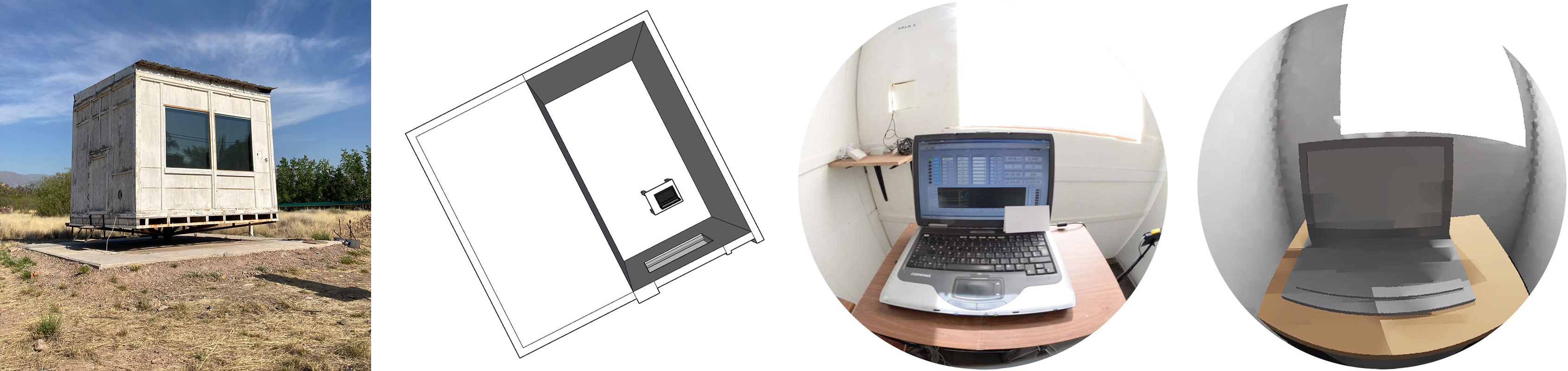
Fig. 1. Facade, floor plan and visualization of the real and Radiance simulated environment of the Lighting Research Laboratory - CONICET CCT Mendoza.
2.2. Daylight simulation
2.2.1. Geometry
The 3D model for this space was generated with Trimble SketchUp Make v.2015 (without support since 2020). This software works on ruby language code, an interpreted, reflexive and object oriented programming language which allows users to generate program sectors to modify its functionality. Within this language code, the extension Warehouse Groundhog [27] Open Source v.3 was used to export 3D models to the Radiance framework [28], which is a high accuracy ray-tracing software considered one of the most powerful lighting simulation tools with wide validation over the last 20 years [29].
2.2.2. Materials
The luminances of the predominant materials in the environment (walls, floor, roof and workspace) were determined to characterize them from their reflectances in the virtual model. These in situ measurements were carried out according to the measurement protocol of Fontoynont [30]. The instruments used were a Minolta LS 110 luminance meter (calibration certificate, reading angle of 1/3° and measuring range of 0.01 to 999,900 cd/m2 and Kodak standard charts. The optical characteristics of the architectural surfaces are reported in Table 1. In addition, glass surfaces were characterized as: clear glass (4 mm), the optical characteristics (0.89 visible transmittance, 0.08 reflectance) were imported from a file (*.rad) generated by the OPTICS software. In this computer program, a specific description of the materials can be found according to the parameters required by the Radiance environment.
Table 1
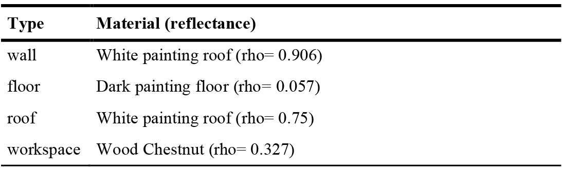
Table 1. Materials reflectance values used in Radiance.
2.2.3. Climate file
The simulations were carried out using the ARG_MendozaCCT (land stations data) weather data file corresponding to the city of Mendoza. This database was generated based on the information provided by the daylight measurement stations of the INAHE, located in the Science and Technology Center, Mendoza (32° 53' S y 68° 52' O) [31]. The sky condition was defined using the Perez model and feeding the gendaylit33 function, deriving the radiation values from the same weather file used in the annual simulation. According to LEED v4, the radiation input for a point in time is the average of the hourly value of two days within 15 days of the equinoxes and solstices.
For this study, 324 simulations (3 season, 3 orientations and 36 -periods of time- intervals of 15-minutes between 8 and 16:45) were carried out. These analyzed conditions correspond to the combination of the following variables: (i) orientations: 90º W (o_west), 180º N (o_north) and 270º E (o_east), which were defined in degrees according to the azimuth of the window. The South orientation (0º South) was not simulated due to the scarce direct solar light contribution of the south hemisphere. (ii) The glare analysis was performed generating point-in-time simulations for the three typical days from the main seasons: 21st of September (equinox), 21st of December (summer solstice) and 21st of June (winter solstice) for each fifteen minutes during working hours, from 8:00 to 16:45. (iii) Space occupation: continuous working day employed in commercial and administrative offices. The adaptation in space occupancy that ends at 16:45 -and not at 17:00- is to maintain symmetry and coherence in the times of the day. It is divided in three phases according to the times of the day (TD): morning: 8:00-10:45; noon: 11:00- 13:45 and afternoon 14:00 – 16:45 [22] in order to reach a better understanding of the results.
2.2.4. Glare metric
First, a point of view of interest is chosen that corresponds to the position of the occupant in space (Fig. 1), then renderings should be produced in the Radiance [33] image format. The rpict command is used to generate an image from the given Radiance scene in octree and send it to the high dynamic range (*.hdr) image in hemispherical fisheye view. The parameters used correspond to the accuracy scene described by Jakubiec [34] (ab) 5; (ad) 2048; (as) 512; (aa) 0.08; (ar) 512; (dt) 0; (ds) 0. Finally, a glare assessment should be performed using the Radiance sub-program evalglare [35,36]. Daylight glare probability (DGP) model was selected for the glare analysis. This model presents the best performance and robustness in relation to other available metrics [15]. Wienold J. [36] developed the pre-processing tool evalglare for RADIANCE to calculate not only the DGP, but also the other commonly used glare metrics, based on HDR images originating from luminance distribution measurements or simulations. DGP calculated from two terms within its Eq. (1) [17]: (a) vertical eye illuminance, as the main parameter within the equation since it is the variable which best correlates with glare perception [19] and (b) luminance relations, size and source position calculated from the HDR.
Table 2
![Cut-off values for both models for the 4-point scale: DGPW [15] and DGPB: Morning: 8:00–10:59; noon and afternoon: 11:00 a 17:00 Bian et al. [22]. Ordinal and dichotomous re-codified variables.](figures/8-284-7.jpg)
Table 2. Cut-off values for both models for the 4-point scale: DGPW [15] and DGPB: Morning: 8:00–10:59; noon and afternoon: 11:00 a 17:00 Bian et al. [22]. Ordinal and dichotomous re-codified variables.
Based on the obtained DGP values, two new variables are generated through a re-codification process. The first one is an ordinal variable considering the 4-point scale and the cut-off values determined by Wienold & Christoffersen [15] (DGPW) and Bian et al. [22] (DGPB Morning y DGPB Noon-afternoon): (1) imperceptible; (2) perceptible; (3) disturbing and (4) intolerable (Table 2). The second one is a dichotomous variable of absence and presence of glare. In order to do this, cut-off categories (1) and (2) within the absence of glare and (3) and (4) within the presence of glare were considered. Table 1 shows the values, variables and criteria mentioned above.
Below is a flowchart (Fig. 2) with the simulation processes involved in the described methodology. Its beginning with the geometry, materials and climate files (Radiance input files) until obtaining the DGP according to the proposals of Wienold [15] and Bian [22] (output files).
Figure 2
![Cut-off values for both models for the 4-point scale: DGPW [15] and DGPB: Morning: 8:00–10:59; noon and afternoon: 11:00 a 17:00 Bian et al. [22]. Ordinal and dichotomous re-codified variables.](figures/8-284-2.jpg)
Fig. 2. Cut-off values for both models for the 4-point scale: DGPW [15] and DGPB: Morning: 8:00–10:59; noon and afternoon: 11:00 a 17:00 Bian et al. [22]. Ordinal and dichotomous re-codified variables.
2.3. Statistical analysis
Once the continuous DGP values were obtained, the following actions were carried out: (i) Statistical analysis of DGP values according to time of the day (TD) -morning, noon and afternoon-. This study analyze and compare the behavior of DGP values in the course of the day for the different orientations and seasons (spring, summer and winter). (ii) Disparity occurrence analysis in the categorization of DGP values. This categorization was made according to the cut-off criteria proposed by both authors (see Table 1). The disparity occurrence is analyzed among these categories (∆CAT) and their percentage during the day (%∆CAT) is calculated for the different conditions. Finally, (iii) Disparity Occurrence Analysis in the threshold of Absence-presence of glare. In contrast to the previous analysis, this one re-codifies DGP values within the dichotomous variable of absence (DGP < 0.38) or presence (DGP > 0.38) of glare in which the occurrence of disparity is analyzed between both authors’ categories (∆CAT) and their percentage during the day is calculated (%∆CAT).
3. Results
3.1. Statistical analysis of DGP values by times of the day (morning, noon, afternoon)
West Orientation (o_west): As Table 3 shows, the o_west shows a similar behavior to the o_north with a gradual increase in the DGP values along the day and an opposite behavior regarding the o_east. This means that, in this orientation, DGP values increase from morning to afternoon. When analyzing the seasons, it can be observed that during the mid-season, morning values begin in no glare condition (DGP 0.31), remain steady at noon (DGP 0.33) and increase in the afternoon reaching a DGP value of 0.55. As shown in the box plot (Fig. 3), mornings and noon periods along all seasons present no glare conditions, with spring and winter mornings displaying the main dispersions, reaching DGP values of 0.03 and 0.09 respectively. However, the main dispersions along the day take place during the afternoon periods along all seasons with SD values reaching 0.15, 0.07 and 0.17 in spring, summer and winter, respectively. When going deeper into the analysis of afternoon periods along all seasons, the lower and upper quartiles are within glare values (DGP > 0.38).
Table 3
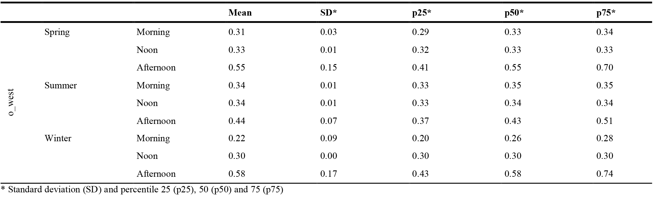
Table 3. DGP values for the west orientation (o_west) for typical spring, summer and winter days for the different TD.
Figure 3
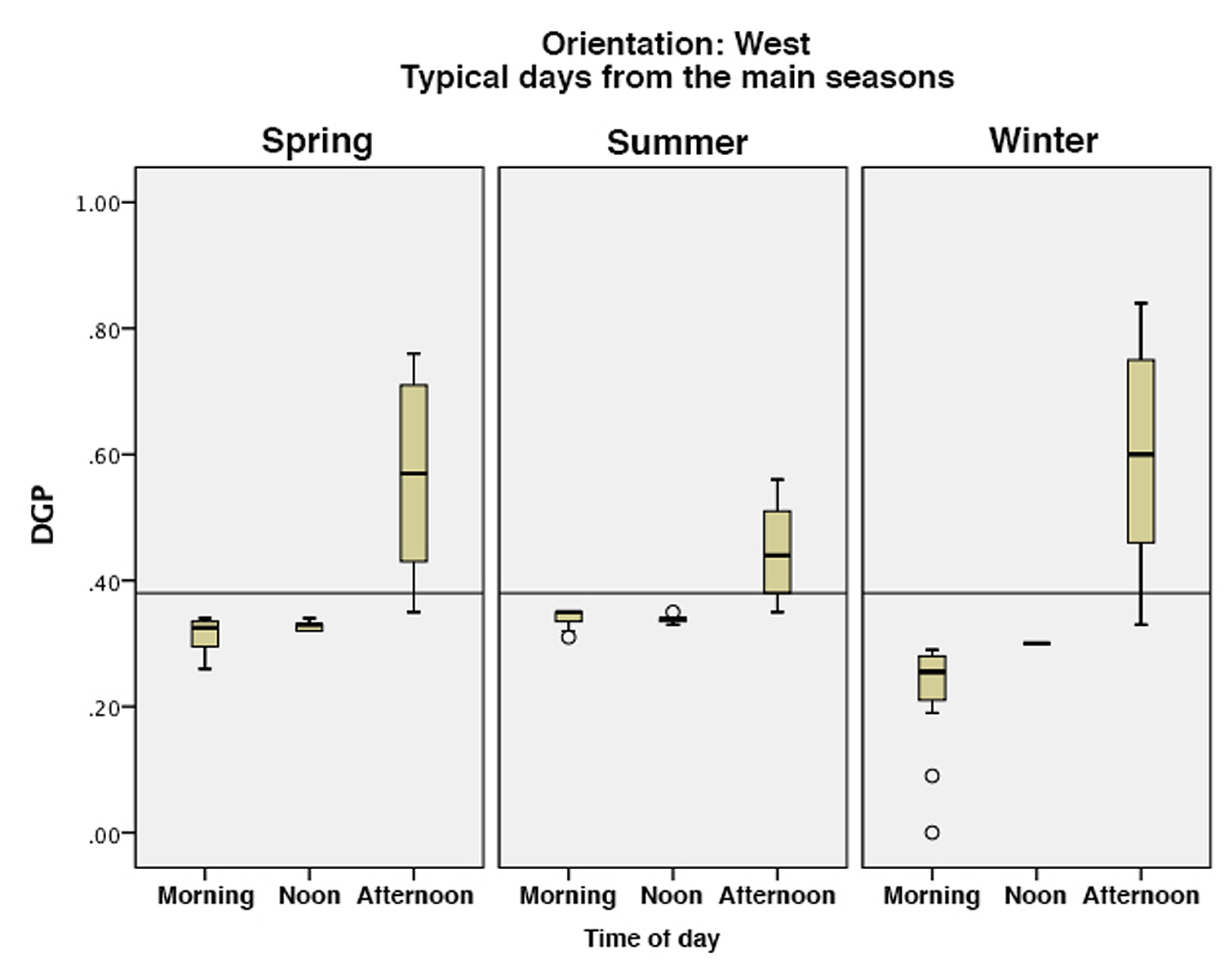
Fig. 3. Box plot of DGP values for o_west on typical seasonal days in different times of day.
North Orientation: (o_north). Opposite to the o_east, the o_north shows a gradual increase -as explained later- of the average DGP values along the day (Table 4 and Fig. 4). When running a seasonal analysis of the results, it is observed that, during spring, morning registers start in glare conditions (DGP 0.44) and increase along the day reaching a maximum value during the afternoon (DGP 0.54). During the summer, the different times of the day are under no glare conditions with a lower dispersion when compared to the rest of the seasons. Finally, in winter the main variations in this orientation are found during all the TD, presenting values such as DS 0.3, 0.21 and 0.13 for morning, noon and afternoon, respectively. When it comes to spring, a major dispersion with DS value 0.13 is observed, with an upper quartile within glare condition (DGP 0.56) and a lower quartile reaching the boundary of no glare (DGP 0.32).
Table 4
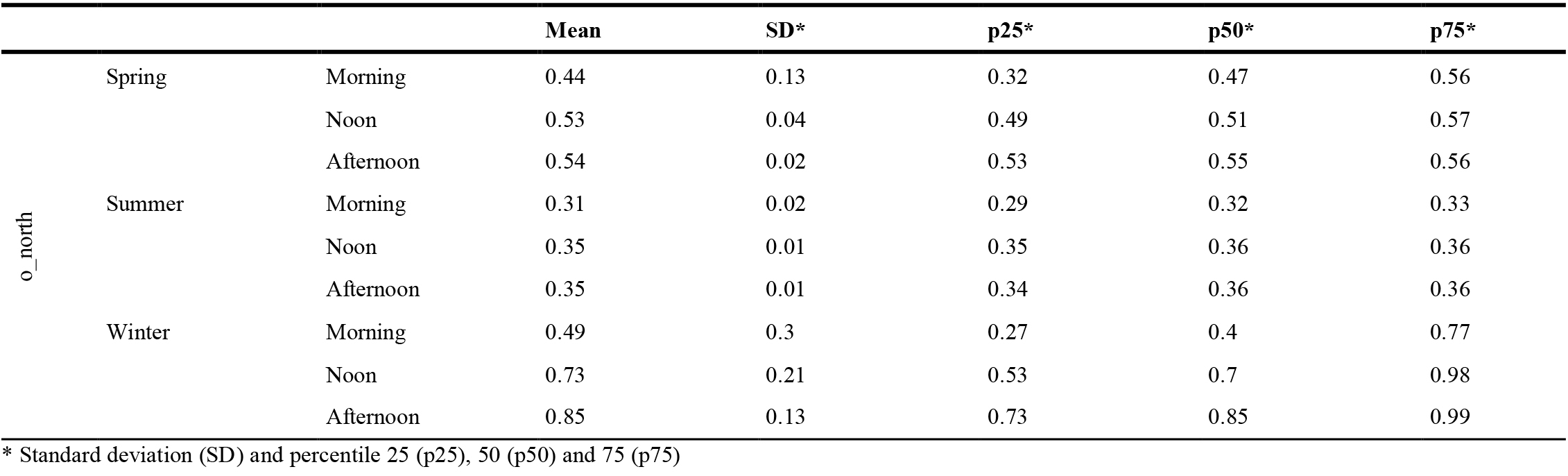
Table 4. DGP values for the north orientation (o_north) for typical spring, summer and winter days for the different TD.
Figure 4
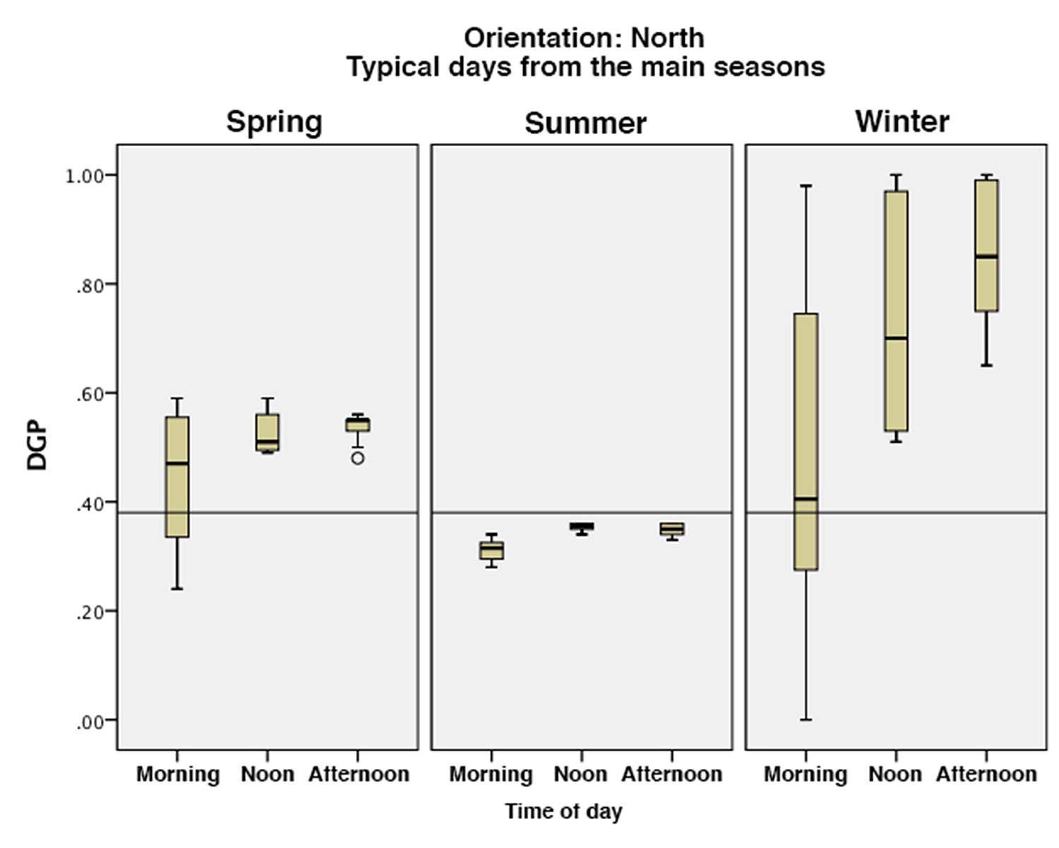
Fig. 4. Box plot of DGP values for o_north on typical seasonal days in different times of day.
East Orientation (o_east): In this orientation, average DGP values present a similar behavior along the different seasons analyzed, with a decrease along the day. This means that the registered values in the morning begin with DGP > 0.5 and decrease to DGP values between 0.42 and 0.46 at noon, reaching DGP values of 0.3 and 0.35 in the afternoon (Table 5 and Fig. 5). Even though mornings start with different DGP values along all seasons, these unify as the day passes by. When seasonally analyzing the average results obtained in this research, it is observed that during spring, morning registers begin in a critical glare condition (DGP 0.97) which decreases along the day until reaching its minimum value during the afternoon (DGP 0.33).
Table 5
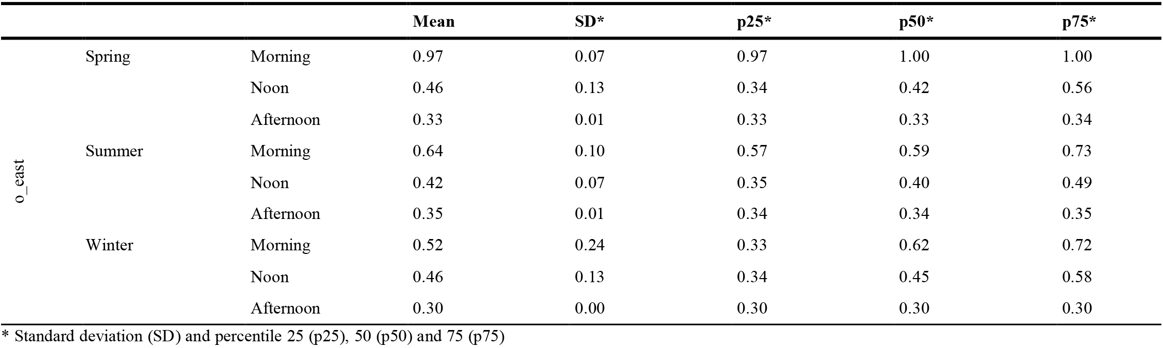
Table 5. DGP values for the east orientation (o_east) for typical spring, summer and winter days for the different TD.
Figure 5
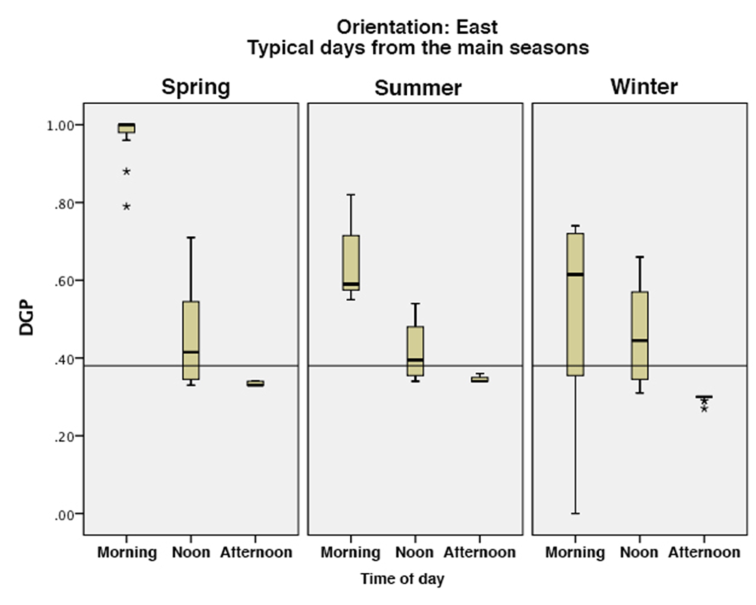
Fig. 5. Box plot of DGP values for o_east on typical seasonal days in different times of day.
3.2. Disparity occurrence analysis in the categorization of DGP values (ordinal) for full day and times of the day (morning, noon and afternoon)
Table 6 shows that regarding the o_east, summer is the season with major discrepancy occurrence (∆CAT) showing a daily percentage of 37.84% (14 discrepancy occurrence out of the 37 conditions) while in spring and winter this percentage does not exceed 6%. Similarly, it can be observed that there was an underestimation of Bian’s proposed DGP in all cases. This means that when comparing the data categorized by the two models, the cut-off points proposed by Bian in the DGP usually give a lower category than that obtained by the model proposed by Wienold (original model). On the other hand, in the o_north, summer stands out again with the highest disparity, 64, 86% (24 out of the 37 conditions). In opposition to the o_east, spring and winter do not exceed 2% of the day. In this case, it is important to highlight that the percentage difference found is 64.86%, of which 79.17% of them present an overestimation. Finally, the o_west shows that a disparity concentration is perceived in the mid-season period and in summer with 18.92% and 24.32%, respectively. In keeping with this, these differences are underestimated by 85.71% in spring while in summer time they are overestimated 77.78% of the cases.
Table 6
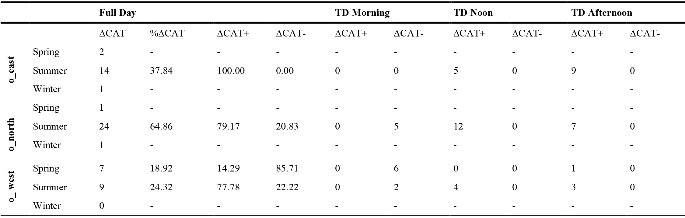
Table 6. Discrepancy occurrence (∆CAT), overestimations (∆CAT+) and underestimations (∆CAT-) between both models (ordinal) for the different orientations, seasons (spring, summer and winter) and TD.
In order to deepen the analysis, the TD are analyzed on the basis of these conditions. Overestimations are registered in the results of the o_east in the summer, during noon and the afternoon, with percentages reaching 64.28% and 35.71%, respectively. This shows that, during the summer season, the main overestimated differences are found in the afternoon (14:00 -16:45). In the o_north, during the summer, a noon overestimation is found with a percentage of 50% and underestimations during the morning and afternoon of 20.83% and 29.16%, respectively. This means that half of the differences registered during the day are found at noon with an underestimation of Bian DGP values, while the other half is found during the morning and afternoon with an underestimation of these values. Finally, in the o_west during spring, 85.71% of the underestimation is found during the morning, while in summer, 77.77% of the overestimation is found between noon and the afternoon.
3.3 Disparity occurrence analysis in glare prediction
In order to analyze the impact of this gap in glare/no glare predictions, a new analysis with the DGP values was carried out which consisted in a dichotomous categorization of DGP values by means of a 0.38 cut-off value. By doing so, DGP values < 0.38 are under conditions of no glare while those DGP> 0.38 are within conditions of glare. The glare prediction difference (dichotomous) was lower than 2.7%. The main annual differences were registered in the o_west (summer) and o_east (spring, and winter) with a 2.7% (Table 7). Similarly, in all cases, these differences present an underestimation of Bian’s model which was only found at noon, more precisely at 12.30 during midseason period and summer, and at 12.45 during winter. On the other hand, the afternoon presented a lower difference in the o_west during summer time, more specifically at 15:00. This low difference could be justified by the time criterion proposed by Bian et al. [23] -no later than 17:00- even though simulation registers for these latitudes show glare conditions up to 19:00 approximately.
Table 7
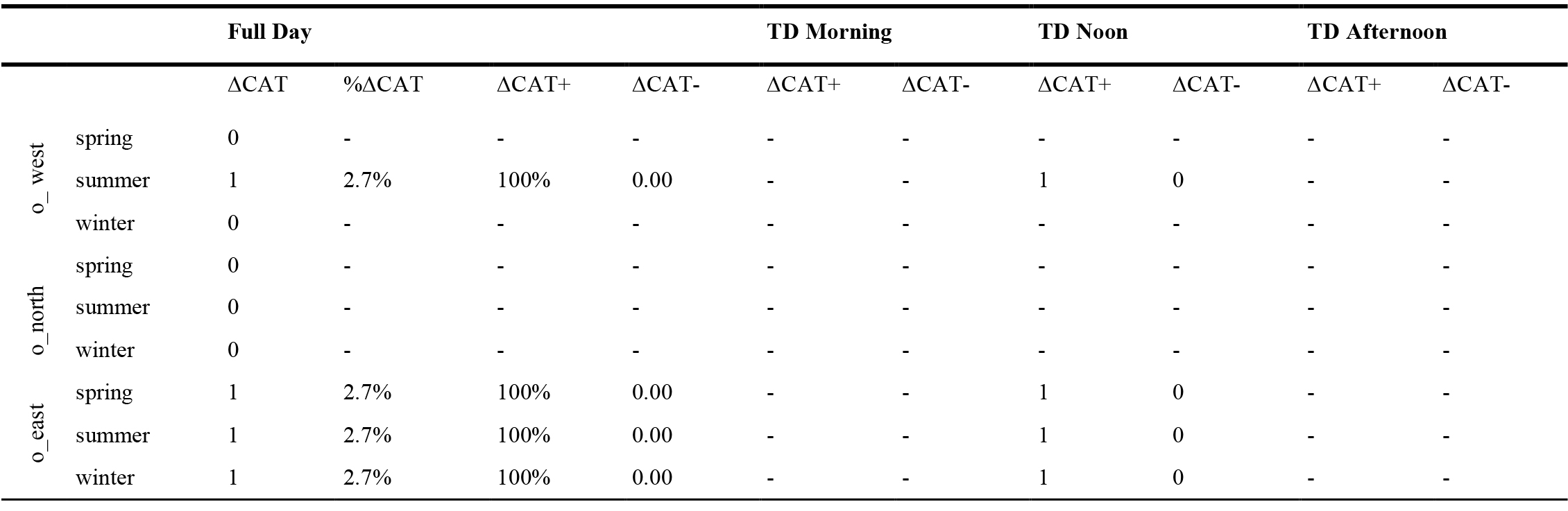
Table 7 Discrepancy occurrence (∆CAT), overestimations (∆CAT+) and underestimations (∆CAT-) in glare prediction (dichotomous) between both models for the different orientations, seasons (spring, summer and winter) and TD.
4. Discussion
This research allowed a more in-depth analysis of the complexity of the glare factor in more than 300 daylight conditions in a bright climate with a predominantly clear sky and the application of two current cut-off points of DGP [15,22] model.
In the first statistical analysis, it was possible to characterize the DGP in the different conditions. The results showed that every orientation along the year presents a similar behavior in relation to glare values. This means that every orientation presents characteristics which remain steady in the different seasons, showing that, for example, while the o_west and o_north present an increasing behavior in DGP values from morning to afternoon, in the o_east, this is completely opposite. According to solar geometry, this opposing behavior is predictable, however, after analyzing the distribution of DGP values, the o_east presented a wider daylight dispersion in contrast to the o_west. It is expected that future studies will adjust daytime hours and space occupation hours in order to extend the hours of analysis based on bright climates with greater availability of hours of sunshine. Based on the registered behaviors and considering 0.38 as cut-off value (glare absence/presence), the most critical times of the day (TD) - morning, noon, and afternoon- were: o_west/afternoon, o_north/morning and afternoon and o_east/morning and noon. Similarly, it was possible to analyze the dispersion and to highlight the o_north since: (i) the winter season was the most critical due to the high recorded values and the high variability in every TD, and (ii) the summer season presented the most stable and less varied TD values.
In the second stage, the occurrence of disparities in the ordinal characterization of DGP values was analyzed. Results showed an important gap between the two proposals reaching differences of up to 64.86%. No disparities higher than a category were observed in the analyzed conditions. The main differences were found during the summer period with an average of 42.07% for the different orientations, followed by spring and winter with a 9.01% and 1.8% respectively. Finally, regarding the TD, the main differences were found during noon and the afternoon with an underestimation of the DGPB values while during the morning, an underestimation was registered mainly for the west orientation in spring. However, if we analyze the difference in glare prediction on the dichotomous scale (presence / absence of glare) it was less than 2.7%, a relatively low difference between the two cut-off points tested.
Even though the new proposed cut-off values (DGPB) were able to quantify and provide a concrete value to the impact of time over glare sensation, this research found some aspects which are worth considering and reflecting upon. On the one hand, previous studies [17,18], found that certain variables (fatigue, consumption of certain foods such as caffeine, chronotype, prior exposure to a light source, sky condition) related to glare response according to the time of the day have not been considered. On the other hand, in spite of the fact that the results obtained from the analyzed conditions could suggest that the differences found in the ordinal scale were considerable, but not in the dichotomous scale. This would be an early statement since deeper studies show that their impact on glare prediction is minimum.
5. Conclusion
This work has enabled the application of two currently available 4-point scale proposals in simulation environments. The main objective of this work was to compare the DGP model (original cut-off values) with new cut-off values that differ according to the time of day (morning, noon and afternoon). These two cut off values were compared at more than 300 simulated conditions. Two main results are presented in this study. On the one hand, the performance of the DGP model by orientation and by time of day (morning, noon, afternoon) in the simulated scenarios and on the other hand and as a main result, the analysis of disparity occurrence in the glare prediction of the two cut-off values of the DGP model. Specifically, this result showed that the glare prediction difference (in a dichotomous scale) was lower than 2.7%. In other words, a relatively small difference.
This work is not without limitations. (i) The complexity of the study of the dynamic behavior of daylight (dynamic source that fluctuates in color, intensity, direction and availability) and its validation in simulation environments, the typical space of an office box was recreated in a Lighting Research Laboratory. (ii) The study was only focused on one point of view; however, the criterion is based on “the worst case scenario” as mentioned in EN 1450140 in cases of multiple available activity positions. (iii) Technical and equipment limitations made continuous monitoring data from the lab is impossible. (iv) Reduced number of simulations. These limitations mean that the results must be contextualized to the simulated conditions, so they cannot be generalized to other daylighting conditions, populations, climates (sky condition) and views. In that sense, validation of such thresholds should be complemented with studies currently underway. DGP cut-off values are critical when it comes to human comfort in spaces with daylight conditions. In future work, it is planned to evaluate the subjective response of people at different times of the day to complement the studies carried out to date.
The following questions arise from this research work:
- What about those values close to the cut-off point where even though they do not influence glare prediction, they can offer glare categorization variations higher than 60%. Due to this, it is necessary to go deeper in psychophysical studies to obtain more evidence on people´s glare perception along the day.
- It is also necessary to establish new criteria considering sky conditions. Clear sky, for example, is characterized by a non-uniform luminance distribution and generally presents mean maximum global illuminance values of 90.000 lx in summer and 30.000 lx in winter. This important difference (60.000lx) leads to considering a seasonal analysis for these regions which must be focused on improving predictive tools to be used in the design stages and evaluation of daylight strategies.
- Decisions based on this information will not only affect the quality and quantity of light but also costs, views, solar gain and energy use. In this context, as the different cut-off values proposed by Bian et al.23 for each TD, it is necessary to closely analyze the impact that each season has on users´ glare tolerance and perception. If this is accomplished, it will be possible not only to generate predictive and analysis tools which are more representative of the lighting conditions of a given space but also to perform more efficient interventions.
Contributions
All authors contributed equally in the preparation of this article.
Declaration of competing interest
The authors declares that there is no conflict of interest.
References
- M.G. Figueiro and M.S. Rea. The effects of red and blue lights on circadian variations in cortisol, alpha amylase, and melatonin, Int J Endocrinol. Epub ahead of print 24 June 2010. https://doi.org/10.1155/2010/829351
- R.D. Clear. Discomfort glare: What do we actually know?, Lighting Research and Technology 45(2) (2013) 141–158. https://doi.org/10.1177/1477153512444527
- T. Kruisselbrink, R. Dangol and A. Rosemann. Photometric measurements of lighting quality: An overview, Building and Environment 138 (2018) 42–52. https://doi.org/10.1016/j.buildenv.2018.04.028
- J.Y. Shin, G.Y. Yun and J.T. Kim. Evaluation of Daylighting Effectiveness and Energy Saving Potentials of Light-Pipe Systems in Buildings, Indoor and Built Environment 21(1) (2012) 129–136. https://doi.org/10.1177/1420326x11420011
- M.B. Hirning, G.L. Isoardi and I. Cowling. Discomfort glare in open plan green buildings, Energy Build 70 (2014) 427–440. https://doi.org/10.1016/j.enbuild.2013.11.053
- S. Carlucci, F. Causone, F. De Rosa and L. Pagliano. A review of indices for assessing visual comfort with a view to their use in optimization processes to support building integrated design, Renew. Sustain. Energy Rev. 47 (2015) 1016-1033. https://doi.org/10.1016/j.rser.2015.03.062
- W.K.E. Osterhaus. Discomfort glare assessment and prevention for daylight applications in office environments, Sol. Energy 79 (2005) 140–158. https://doi.org/10.1016/j.solener.2004.11.011
- CIE. 1983. Discomfort glare in the interior working environment. Vienna, Austria: Commission Internationale de l’Eclairage. No. 55:1983. 52p.
- N.S. Shafavi, Z.S. Zomorodian, M. Tahsildoost and M. Javadi, M. Occupants visual comfort assessments: A review of field studies and lab experiments, Solar Energy 208 (2020) 249-274. https://doi.org/10.1016/j.solener.2020.07.058
- J.A. Jakubiec, C.F. Reinhart and K. Wymelenberg Van Den. Towards an integrated framework for predicting visual comfort conditions from luminance-based metrics in perimeter daylit spaces, in: Build. Simul. Conf., 2015, pp. 2–9.
- I. Konstantzos and A. Tzempelikos. Daylight glare evaluation with the sun in the field of view through window shades, Building and Environment 113 (2017) 65-67. https://doi.org/10.1016/j.buildenv.2016.09.009
- J.Y. Suk. Luminance and vertical eye illuminance thresholds for occupants’ visual comfort in daylit office environments, Build. Environ. 148 (2019) 107–115. https://doi.org/10.1016/j.buildenv.2018.10.058
- J. Wienold, T. Iwata, M. Sarey Khanie, et al. Cross-validation and robustness of daylight glare metrics, Lighting Research & Technology 51(7) (2019) 983-1013. https://doi.org/10.1177/1477153519826003
- J. Wienold and J. Christoffersen. Evaluation methods and development of a new glare prediction model for daylight environments with the use of CCD cameras, Energy and buildings 38(7) (2006) 743-757. https://doi.org/10.1016/j.enbuild.2006.03.017
- R.G. Rodriguez, J.A. Garretón and A.E. Pattini. An epidemiological approach to daylight discomfort glare, Building and Environment 113 (2017) 39-48. https://doi.org/10.1016/j.buildenv.2016.09.028
- C. Pierson, J. Wienold and M. Bodart. Discomfort glare perception in daylighting: influencing factors, Energy Procedia 122 (2017) 331–336. https://doi.org/10.1016/j.egypro.2017.07.332
- S. Altomonte, M.G. Kent, P.R. Tregenza and R. Wilson. Visual task difficulty and temporal influences in glare response, Building and Environment 95 (2016) 209–226. https://doi.org/10.1016/j.buildenv.2015.09.021
- M.G. Kent, S. Altomonte, P.R. Tregenza and R. Wilson. Discomfort glare and time of day, Lighting Research and Technology 47(6) (2015) 641-657. https://doi.org/10.1177/1477153514547291
- W.K.E. Osterhaus and I.L. Bailey. Large area glare sources and their effect on visual discomfort and visual performance at computer workstations, in: Industry Applications Society Annual Meeting, 1992, pp.1825–1829. https://doi.org/10.1109/ias.1992.244537
- W.K.E. Osterhaus. (1996). Discomfort glare from large area glare sources at computer workstations, in: Proceedings for the 1996 International Daylight Workshop, Building with Daylight: Energy-Efficient Design, Perth, Western Australia, November 1996, pp.103–110.
- J. Yamin, A. Pattini and E. Colombo. Confort visual en oficinas, factor temporal en la evaluación de deslumbramiento. Informes de La Construcción 72(557) (2020) e329. https://doi.org/10.3989/ic.67992
- Y. Bian, Q. Dai, Y. Ma and L. Liu. Variable set points of glare control strategy for side-lit spaces: Daylight glare tolerance by time of day, Solar Energy 201 (2020) 268–278. https://doi.org/10.1016/j.solener.2020.03.016
- R.A. Mangkuto, K.A. Kurnia, D.N. Azizah, R.T. Atmodipoero and F.X.N. Soelami. Determination of discomfort glare criteria for daylit space in Indonesia, Sol. Energy 149 (2017) 151–163. https://doi.org/10.1016/j.solener.2017.04.010
- J. Yamin Garretón, R.G. Rodriguez, A. Ruiz and A.E. Pattini. Degree of eye opening: A new discomfort glare indicator, Building and Environment 88 (2015) 142-150. https://doi.org/10.1016/j.buildenv.2014.11.010
- Europe Norms, EN 14501. Blinds and shutters. Thermal and visual comfort. Performance characteristics and classification, 2018. https://doi.org/10.3403/30100403u
- A. Villalba, J. Yamín, J. Weinold, J.M. Monteoliva and A. Pattini, Caracterización del comportamiento óptico de cortinas textiles en simulación de iluminación natural, in: Actas del VI Congreso Latinoamericano de Simulación de Edificios IBPSA LATAM 2019, Mendoza, Argentina, October 2019, pp.117-127. https://doi.org/10.1590/s1678-86212014000300004
- G. Molina, S. Vera, W. Bustamante and T. Bleicher. Groundhog - SketchUpExtension for exporting Radiance models, 2008, Available at: https://extensions.sketchup.com/en/content/groundho.
- G. Ward, The Radiance Lighting Simulation and Rendering System, Computer Graphics, in: Proceedings of '94 SIGGRAPH Conference, 1994. https://doi.org/10.1145/192161.192286
- U. Berardi and T. Wang. Daylighting in an atrium-type high performance house, Building and Environment 76 (2014) 92–104. https://doi.org/10.1016/j.buildenv.2014.02.008
- Fontoynont, M. Daylight Performance of Buildings. Lyon: ENTPE, 1999. zzzzzzzzzz
- J.M. Monteoliva, A. Villalba and A. Pattini. Variability in dynamic daylight simulation in clear sky conditions according to selected weather file: Satellite data and land-based station data, Lighting Research & Technology 49 (2015) 508–520. https://doi.org/10.1177/1477153515622242
- C.F. Reinhart and K. Voss. Monitoring manual control of electric lighting and blinds, Light. Res. Technol. 35(3) (2003) 243–260. https://doi.org/10.1191/1365782803li064oa
- G.L. Ward and R.A. Shakespeare. Rendering with Radiance, Morgan Kaufmann Publishers, 1998, Revised edition 2007, ISBN 0-9745381-0-8.
- J.A. Jakubiec and C.F. Reinhart. The 'adaptive zone' - A concept for assessing glare throughout daylit spaces, Lighting Research and Technology 44 (2012) 149-170. https://doi.org/10.1177/1477153511420097
- J. Wienold, Evalglare: A new Radiance-based tool to evaluate glare in office spaces, in: 3rd International Radiance Workshop, 2004.
- J. Suk and M. Schiler, Investigation of Evalglare software, daylight glare probability and high dynamic range imaging for daylight glare analysis, Light. Res. Technol. 45 (2013) 450–463. https://doi.org/10.1177/1477153512458671
Copyright © 2021 The Author(s). Published by solarlits.com.

4681
Total views
Citations
SHARE ON


