Volume 8 Issue 1 pp. 86-99 • doi: 10.15627/jd.2021.6
An Intelligent IoT-enabled Lighting System for Energy-efficient Crop Production
Jun Jiang,*,a Mehrdad Moallem,*,a Youbin Zhengib
Author affiliations
a School of Mechatronic Systems Engineering, Simon Fraser University, BC, Canada
b School of Environmental Sciences, University of Guelph, ON, Canada
*Corresponding author.
alex_jiang_2@sfu.ca (J. Jiang)
mmoallem@sfu.ca (M. Moallem)
yzheng@uoguelph.ca (Y. Zheng)
History: Received 03 October 2020 | Revised 22 December 2020 | Accepted 11 January 2021 | Published online 15 February 2021
Copyright: © 2021 The Author(s). Published by solarlits.com. This is an open access article under the CC BY license (http://creativecommons.org/licenses/by/4.0/).
Citation: Jun Jiang, Mehrdad Moallem, Youbin Zheng, An Intelligent IoT-enabled Lighting System for Energy-efficient Crop Production, Journal of Daylighting 8 (2021) 86-99. https://dx.doi.org/10.15627/jd.2021.6
Figures and tables
 Figure 13
Abstract
In this paper, an intelligent lighting instrumentation and automation system is presented with the objective of achieving high energy-efficiency in greenhouse supplemental lighting based on the Internet of Things (IoT) technology. The system runs on a Raspbian operating system which interacts with wireless-enabled light emitting diode (LED) fixtures for plant growth, an online data server, and different light sensors including RGB and quantum sensors. The communication is achieved through RestFul API, UART, and I2C. The system is utilized to implement a feedback controller that automatically adjusts the light dimming levels and, in particular, the ratio of red and blue light intensities based on the plants’ needs. A series of experiments involving plant growth were conducted which indicate that the proposed system can achieve energy-savings up to 34%, when compared to a conventional time scheduling scheme. Additionally, the experiments demonstrate that the system can achieve a highly uniform light distribution under unpredictable natural lighting conditions while saving energy due to supplemental lighting.
Keywords
Lighting system instrumentation, Daylight harvesting, Photosynthetic photon flux density, Greenhouse automation
Nomenclature
| IoT | Internet of Things |
| LED | Light Emitting Diode |
| RGB | Red, Green, Blue |
| UART | Universal Asynchronous Receiver/Transmitter |
| I2C | Inter-Integrated Circuit |
| UV | Ultraviolet |
| PPFD | Photosynthetic Photon Flux Density |
| GUI | Graphical User Interface |
| PAR | Photosynthetically Active Radiation |
| HPS | High-Pressure Sodium |
| PWM | Pulse-Width Modulation |
| DLI | Daily Light Integral |
| MCU | Microcontroller Unit |
| ADC | Analog-to-Digital Converter |
1. Introduction
Lighting technology has been well developed for the use in residential and office buildings [1-3]. The research on how to use lighting in the field plant production and animal farming has been increasing during the past several decades [4]. In farm animal production, light treatment has been utilized to improve rearing conditions [5]. For example, studies have shown that supplemental light treatment increased the weight and milk yield in cattle [6]. An lighting environment with optimal combination of light intensity and photo-period has been proven to improve the welfare and behavior of pigs in terms of defecation [7]. Moreover, compared to conventional incandescent lamps, LED lighting is known to offer advantages in terms of feed conversion, production, and welfare [8]. In the area of indoor horticulture, the use of lighting for improving plant growth has been studied using different ratios of light wavelengths and light intensities on different plant species [9]. Studies have shown that the growth results were different depending on plant species, even when similar light treatments were utilized [10,11].
LED supplemental lighting has attracted growing interest in the agriculture sector because of offering a relatively high energy-efficiency and the capability for automated dimming [12-15]. The flexibility to control light at a specific spectrum such as red, blue, and UV can have a positive influence on plant growth and their nutritional content [16-19]. With rapid technology advancements in the field of the Internet of Things (IoT) and wireless communication, smart LED supplemental lighting systems can play a significant role in improving the performance of future intelligent greenhouses [20-22].
In a conventional greenhouse management system [23], the central control unit runs a combination of time scheduling and threshold-based control schemes to maintain a good growing environment for different plants. In particular, environmental factors such as CO2, soil moisture, humidity, temperature, and light intensity have to be maintained at desired levels depending on the specific requirements of the plants [24,25]. By setting a specific time schedule and a threshold range, the sensor and control equipment are triggered at appropriate times.
Research on optimization and improvement of greenhouse systems for supplemental lighting has attracted attention in recent years [26-29]. Greenhouse farming utilize sunlight and supplemental lighting (e.g., from LED fixtures) to deliver uniform light for plant growth, especially during the fall and winter seasons. In [30], the authors demonstrated that a specific ratio of red and blue, achieved through LED supplemental light, can increase the dry weight of pea shoots by increasing photosynthetic photon flux density (PPFD) in the winter’s dark months. In [31] a single-input single-output control method was proposed that used a photosynthetically active radiation (PAR) meter to monitor the PPFD from sunlight to adjust the dimming levels of LEDs. Considering the relatively high cost of PAR-meters, it would be relatively expensive to incorporate them into a large-scale greenhouse. Also, the uniform distribution of light would be an issue. An open-loop control ON-OFF strategy for lighting and shading was discussed using high pressure sodium lights (HPS) in [26,32] to achieve constant daily light integrals (DLI). In [33], an ON-OFF lighting control scheme was presented for high-pressure sodium (HPS) lights based on real-time weather forecast and electricity price. However, an ON-OFF scheme is disadvantageous when it comes to maintaining lighting uniformity. Furthermore, HPS light sources have lower energy efficiency than LEDs [34,35], and not good for frequent on-off operation.
The main focus of this work was the development and implementation of an energy-efficient lighting control system and its experimental evaluation on a proof-of-concept system using real plants. The effect of light treatments on plant growth is not within the scope of the work. Automatic control of lighting can provide greenhouse operators with a variety of advantages. For instance, customized light recipes (e.g., with different ratios of red, blue and UV light) can affect plant growth and phytochemical contents. In this paper, an IoT based measurement and automation system that utilizes Wi-Fi communication with RESTful API is presented for growing micro-greens and compared with conventional ON-OFF methods. The results indicate that the automation platform would allow implementation of sensor-based feedback algorithms that can regulate important variables such as PPFD at plant canopies to meet the DLI requirement while minimizing energy consumption. The organization of this paper is as follows. The IoT-based automation platform is introduced in section 2. In section 3, the model identification and its control system are introduced. Experimental results are presented in section 4 for lighting control which demonstrate the capability of the proposed control system to achieve energy-savings. Conclusions and future work are presented in section 5.
2. IoT system architecture
A small-scale indoor plant growth system was built using LED supplemental lighting fixtures and other sensor modules. The system is equipped with different sensors such as RGB, UV index, PAR quantum, temperature, humidity, soil moisture, and camera. Other components of the system include a microcontroller unit, LED supplemental light fixtures, communication hardware, and a cloud data server. Specific details about this system are presented in the following.
2.1. Small-scale indoor garden set-up
As shown in Fig. 1, the system was built on a 2 ft by 4 ft flood table, assembled with an active aqua tray stand and a 50-gallon capacity reservoir. An Ebb and Flow hydroponic system was built for irrigation and nutrient delivery including a standard water pump, air pump, and timer. The plant growth system was placed in an indoor space facing the south-west direction alongside a transparent french window in order to achieve maximum sunlight exposure (geo-location: N: 49◦11114.411, W: 122◦50159.411.
Figure 1

Fig. 1.Plant growth prototype equipped with an intelligent lighting system.
2.2. Environment monitoring system
The proposed IoT-based measurement and control system is shown in Fig. 2, which consists of the following components:
Figure 2
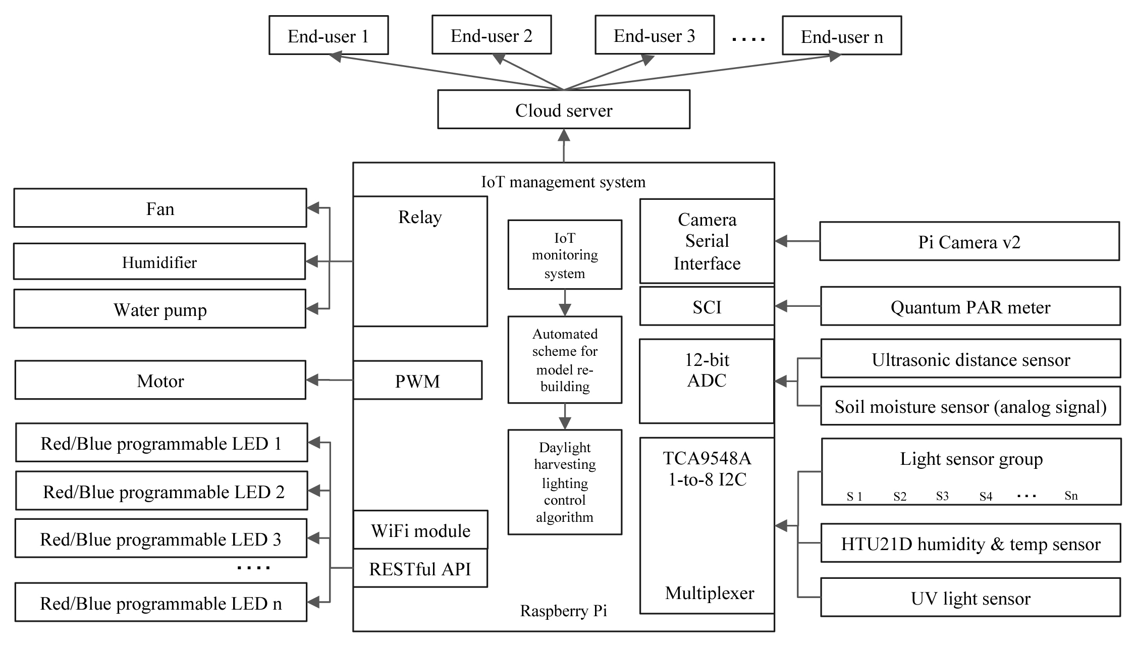
Fig. 2.Schematic diagram of the proposed IoT-based management and control system.
- Daylight monitoring and data acquisition: Lighting data, consisting of combined daylight and supplemental light, were measured by using a group of RGB light sensors TCS34725 (from TAOS, ), quantum sensor MQ-501 (from Apogee Instruments, Inc.), and UV light sensor SI1145 (from Silicon Laboratories). The spectrum responses cover 440nm -485nm on blue channel, 490nm-560nm on green channel, 600nm-670nm on red channel for the RGB light sensor and ultraviolet A/B for the UV light sensor. Figure 3 shows the overall set up of the sensors and the main controller prototype board. Four units of RGB light sensors were installed on each side of the flood tray to collect the combined light intensity coming from the sunlight and LED light units. This sensor set was used to provide real time lighting intensity for system identification and control processes. A TCA9548A I2C multiplexer was used to allow identical I2C devices to be accessed that run on the same port. This is due to having a limited number of I2C ports on the Raspberry Pi board and the identical I2C address issue. A quantum PAR meter (MQ-501 from Apogee Instruments, Inc.) was mounted on top of the LED fixture to evaluate the control performance by measuring PPFD as a reference. Through the serial communications interface (SCI) protocol, the Raspberry Pi acts as a main controller that requests an average value of PPFD data from the quantum sensor every 30 minutes. All the data were saved in a CSV file on the local drive and transmitted to the cloud server and end users.
- Temperature & humidity and soil irrigation monitoring system: To maintain the temperature and humidity within desired ranges required for plant growth, temperature and humidity sensors HTU210D (from Texas Instruments Inc.) were utilized along with a fan and humidifier. A capacitive soil moisture sensor (from Grove) was utilized to obtain real time soil moisture data. Since there was no analog port on the Raspberry Pi, a base hat with a built-in MCU equipped with a 12-bit 8 channel ADC was integrated with the prototype board to convert the analog signal into
- Plant growth monitoring: A web-based camera was installed as a part of the management system for motion detection and on-site tracking of the plant growth progress. This subsystem was also set up for potential use of image recognition with OpenCV software as part of future development of this prototype. A Pi Camera (Module v2) was attached to the CSI port on the Pi microcontroller and placed on the side batten. The web-based camera monitor and motion detection CCTV system was programmed using Python which automatically captures the time lapse images every one second to share with the end users remotely through the TCP/IP protocol with the data saved on the local
- End user remote access and data storage: A standalone computer running as a data server was set up and connected to the same local network as the main controller. This workstation was used for storing the data collected by the controller, keeping log files, displaying the GUI, and providing remote access. Furthermore, a desktop computer was connected to the Internet for uploading data to a cloud data storage service (for example, by using the Google Drive API) and support for remote access via the Virtual Network Computing (VNC)
Figure 3
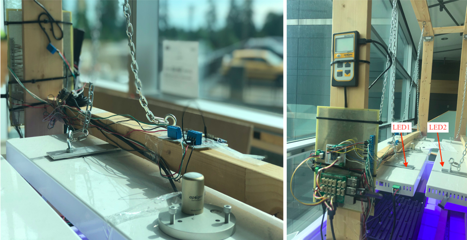
Fig. 3.(a) Quantum PAR meter, UV sensor, and (b) main controller and light sensors.
Since the sunlight intensity varies from one day to another, the water loss from soil would be different on a daily basis. A time-scheduling scheme for the irrigation water pump would not achieve an optimal soil moisture for the plant. To ensure that the soil humidity remains at the optimal level, a relay switch was used for controlling the power of the irrigation pump.
2.3. Wireless supplemental LED fixtures
Two units of wireless controlled LEDs (Q400 from QuantoTech Solutions, Ltd.) were used which allow implementation of features such as tunable red/blue ratios and programmable dimming levels. Both of the LED units were designed for a maximum PPFD output of 480 µmol/s and consist of 7 watts blue LED (460nm), 14 watts red LED (660nm) channel and 2 watts UV LED (385nm). The wireless-enabled LED fixtures in the proposed system were controlled by a Raspberry Pi module through a local WiFi network on the platform using a RESTful API architecture. The WiFi module on each light fixture joins the local network with a self-defined IP address assigned automatically. The Pi controller, connected to the same network, calls for connection with requests library on Python3 platform. Since both light intensity on blue and red channels were dimmable from 0 to 100%, the output of the proposed control system would range from 0 to 1 for blue and red channels, respectively.
The height of the LEDs was adjusted for optimal distance. To this end, a set of experiments were conducted to get the relationship between the height of the LEDs and the effect of the light shading on the plant canopy surface. The height of the LEDs was adjusted from zero (as close to the plant as possible) to 100cm from the plant canopy surface. The PAR sensor and RGB light sensors were both placed near the plants’ canopy surface to record the light data. The steps above were repeated and the dimming levels of the LEDs were adjusted at 20%, 40%, 60%, 80% and 100%, respectively. As shown in Fig. 4, the results indicate that the optimal height is around 17cm-22cm for achieving maximum light exposure from the combination of both LEDs and sunlight.
Figure 4
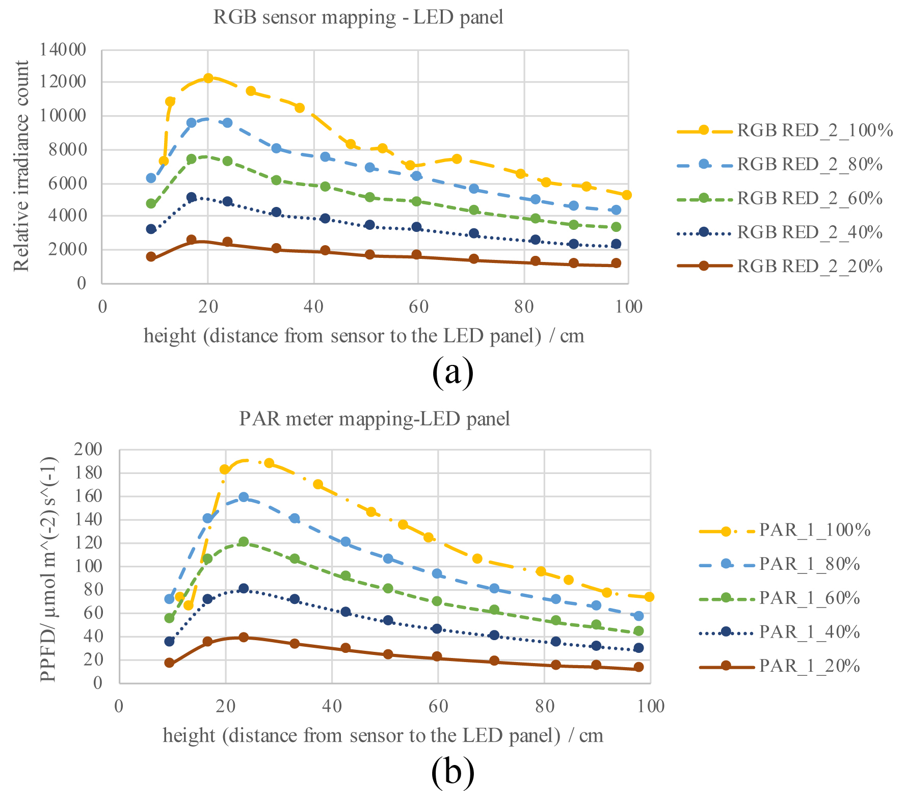
Fig. 4.(a) and (b) Relationship between LED position and light intensity on the plant surface area at different dimming levels.
3. Supplemental lighting control
The proposed lighting system was a linear, static, time-invariant multi-input multi-output (MIMO) system. Research on photometric, electrical, and thermal properties of LEDs, indicate that power consumption has a linear relationship with the LED dimming levels under normal working conditions [37-39]. The performance of a state feedback controller was demonstrated in an indoor grow tent with emulated sunlight environment [36,40]. In this paper, we extended the above work to a real indoor garden exposed to sunlight. In particular, the sky conditions and shade from nearby fixtures can result in asymmetric light exposure on the testbed. For instance, in early mornings and late afternoons, the light distribution in the corner of the setup would result in more shading than the plants located in the center or middle areas.
To tackle the issues mentioned above, certain parameter settings and automation schemes have to be configured. First, a model was obtained using system identification of the lighting environment. Secondly, an automated model identification process was programmed in the controller to update the model on a daily basis. Third, the set point value for both red and blue supplemental light was adjusted along with the plant growth cycle. This is due to the fact that the desired values and ratios of the red and blue lights can vary during different stages of plant growth, depending on the type of plant.
3.1. Control scheme
In the proposed system, daylight is harvested such that minimum supplemental lighting is required from the LED panels. To this end, the total light intensity, which is a combination of supplemental light generated by the LED fixtures and natural light, is measured by light sensors. The system model is given by [40]
where y(t) is the total light intensity at sensor points; yt represents the contribution due to daylight; u(t) is the LED lights dimming input command vector; and T is an m x n full row rank transfer matrix, where m is the number of outputs and n is the number of inputs. The feedback control scheme is based on a state-space linear-quadratic regulator (LQR) method given by (see e.g., [40])
where e(t) = yd-y(t) is the m×1 error vector, with yd being the vector of desired light intensity; and K is the state feedback gain matrix.
3.2. Model identification
As shown in Fig. 3, the LED unit closer to the window is denoted by LED1 and the one farther from window is denoted by LED2. Therefore LED1_R, LED2_R, LED1_B, and LED2_B are defined as the output variables for the red and blue channels on LED1 and LED2, respectively. The identification process, illustrated in Fig. 5, runs after the initialization process on a daily basis. When the disturbance light is at its minimum value, which is usually the case during midnight hours, the system triggers the identification process to obtain the model. This process reduces improves control performance due to variations and disturbance caused by human factors such as changing the locations of sensors or variations in LED light levels. Following a reset of LEDs, RGB sensors S1, S2, S3, ···, Sn record the data when the dimming levels of LEDith are increased from 0% to 100% by steps of 10% (i.e., 10%, 20%, 30%, ···, 100%). The identification process yields matrices such as the following
and
where Tred and Tblue represent the 2 x 2 matrices of the light model (see (1)) in red and blue channels, respectively. Furthermore, control gains Kred and Kblue for the red and blue channels were chosen as follows
and
Figure 5
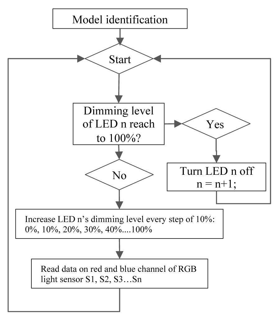
Fig. 5.Lighting system model identification on a daily routine.
3.3. Automated lighting procedure
The automation process includes three main components: IoT monitoring system (Fig. 2), automated scheme for lighting model identification (Fig. 5), and daylight harvesting lighting control (Fig. 6). For each daily system reset, the updated lighting model and control gains were generated and identified as T’ and K’. The value of the desired set-point on red and blue channels were configured and represented as Desired_red’ and Desired_blue’. The system initialization, including the identification and set point selection, only runs once a day. Once the system initialization process is finished, the proposed algorithm acquires sensor data. The data from the red and blue channels of the i-th RGB light sensor were defined as Red 1, Blue 1, Red 2, Blue 2, … Red n, Blue n. The dimming command for the red and blue channels of i-th LED were defined as LED1_red, LED1_blue, LED2_red, LED2_blue, …., LEDn_red, LEDn_blue. The execution cycle runs following the loop procedure as indicated above until the end of the photo-period which is determined by the timer in the main controller. Finally, the system enters sleep mode and turns off the LEDs until next daytime cycle.
Figure 6
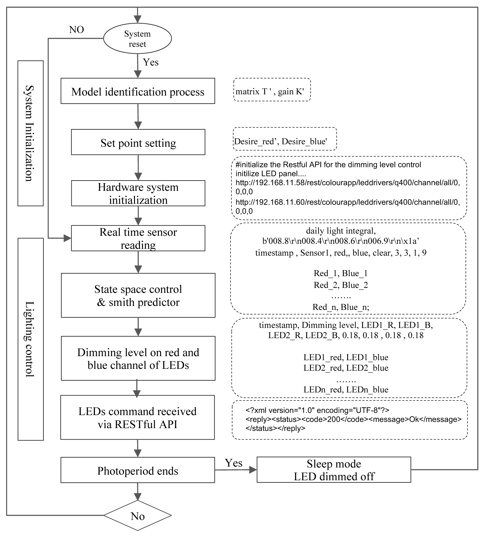
Fig. 6.Process diagram of the proposed IoT management and lighting control system.
4. Experimental results and performance analysis
A series of experiments were conducted from August to November, which cover a broad range of the DLI index from sunlight. To further discuss the system performance, two typical scenarios, including sunny and cloudy days were studied separately. The value of the photoperiod was set as 24 hours in order to evaluate the maximum energy savings and lighting system performance. According to photometric characteristics of the TCS24725 RGB sensor and the fact that the spectral response on the illuminance level varies in a wide range, relative irradiance counts were used as readings taken from both red and blue channels [41,42]. In order to determine the set point value for the system output, calibration was conducted through mapping the counts from the RGB sensor with the data measured from PAR quantum sensor. The desired PPFD was set at 250 µmol m−2 s−1 according to the recommended DLI requirement ranging 13-16 mol m−2 d−1 and photoperiod preference [43,44]. The quantum PAR sensor located on the canopy level of the plant tray, which was the closest location to the examined plants provide the mapping correlation analysis for the RGB light sensors. The desired values for red and blue channels were determined as 3000, 3000, and 3000, 1000 counts, for sunny and cloudy days, respectively. The objective was to evaluate the performance of the daylight harvesting scheme under different red/blue ratios.
As shown in Fig. 7, in sunny days, the plants were exposed to relatively high PPFD from the sunlight, especially during noon and early afternoon. As expected, the data on both blue and red channels of sensor S1, located on the edge of the plant tray, close to the window side, showed that the total light received on the plant surface was over saturated with the peak point reaching over 10,000 counts. Note that the above numbers are sensor data representing relative irradiance counts and do not have any units. A calibration process was conducted with the corresponding values in PPFD units presented later in this section. The data shown for blue and red channels of sensor S4, located on the edge of the plant tray close to the inside of the room, show a relatively smaller amount when saturation occurs. This is due to the fact that there was less sunlight exposed onto the area further from the window than the area closer to the window.
Figure 7
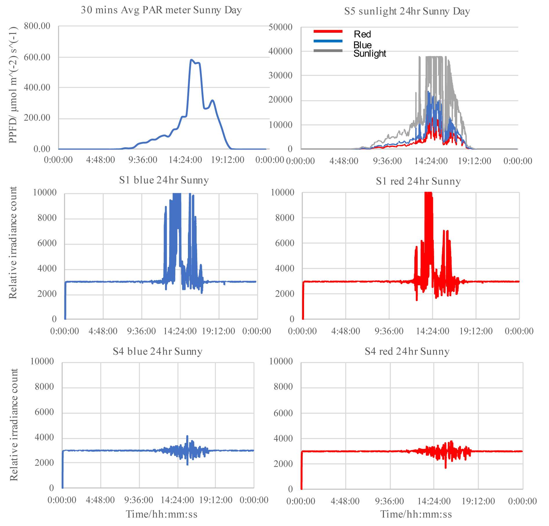
Fig. 7.Sunny day scenario: Daylight variations (top figures), light intensity for blue and red channels of light sensor S1 (middle figures), and sensor S4 readings (bottom figures).
Figure 8 shows the dimming output of the LED1 and LED2 on both red and blue channels in a sunny day. Clearly, LED2 (located further from the window) was dimmed with less fluctuation than the LED1 which was located closer to the window. Specifically, the range of blue and red channels was dimmed between 0.65 to 0.30 and 0.90 to 0.3, respectively, on LED2. The corresponding dimming ranges for LED2, for blue and red, were between 0.8 to 0 and 0.9 to 0, respectively. The data measured by S1 and S4 in Fig. 7 indicate that the combined blue and red light outputs reflected on the plant area were maintained at stable levels, with both achieving the desired set points. Over saturation occurs on both red and blue channels of S1 and S4 during the time from noon peak to early afternoon.
Figure 8
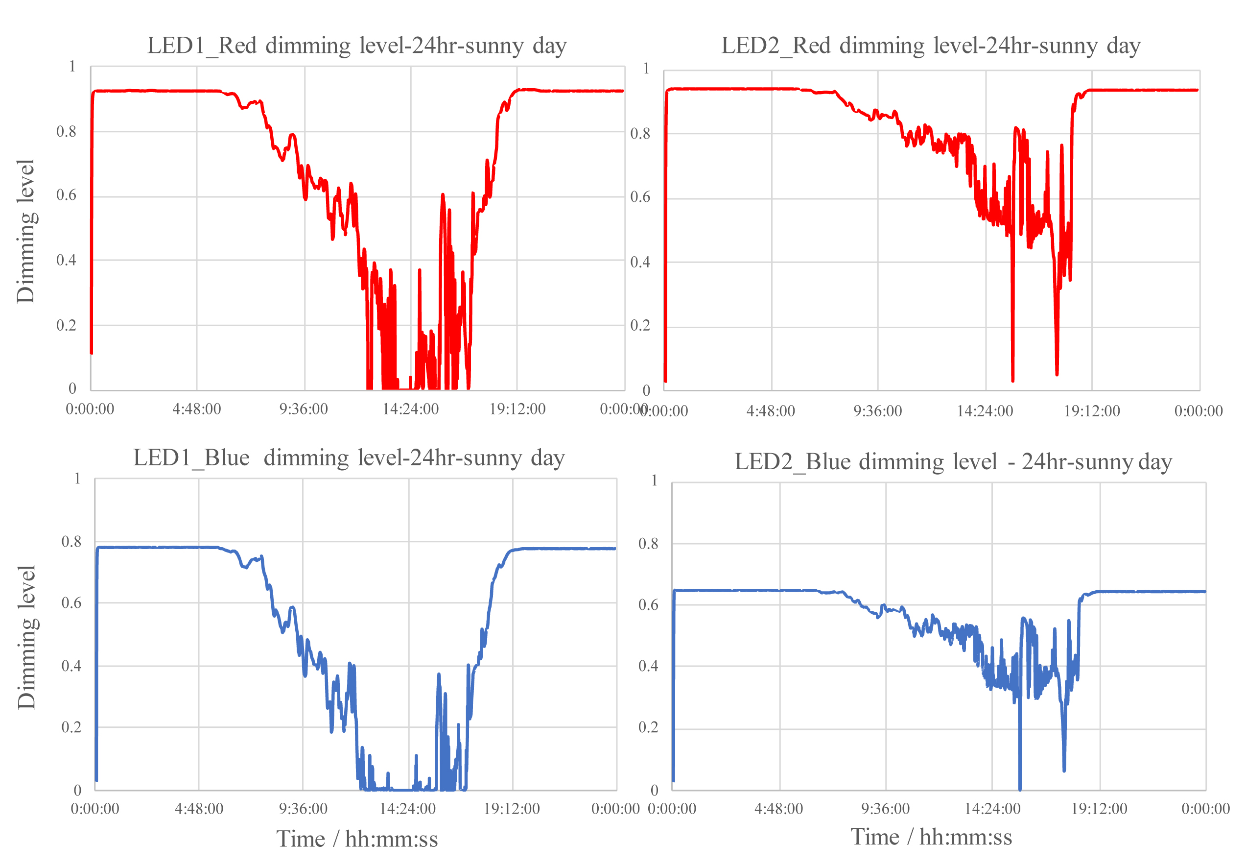
Fig. 8.Sunny day scenario: Dimming level variations in 24hrs for the red and blue channels of LED1 (left) and LED2 (right).
Similarly, the system maintained good performance for cloudy day conditions. A typical cloudy day comes with a relatively low PPFD from the sunlight, while occasionally having randomly strong sunlight exposure during the day. As shown in Fig. 9, the data captured by the PAR sensor and the sensor S5, located on the top of the LED panel to measure the sunlight only, indicate two big disturbances. Specifically, a sudden sunlight drop occurs at 4PM and a sudden sunlight exposure occurs at 5:30PM. Compared with the dimming levels of both LEDs in the sunny day scenario, the LEDs provide more compensation on both red and blue channels, due to less sunlight harvesting in a cloudy day. On the other hand, the total light data recorded on both sensors indicate a smoother curve, especially on the red channel of both S1 and S4. As shown in Fig. 10, both the blue and red channels on LED1 and LED2 act to compensate the light shortage (e.g., resulting in uniform distribution when a sudden shortage of daylight occurs and at 4PM). Also, the light is dimmed down when a large sunlight exposure occurs at 5:30 PM. Overall, the total light exposure at the red and blue channels on both sensors reached the desired set points of 3000 and 1000 counts, respectively.
Figure 9

Fig. 9.Cloudy day scenario: Daylight variations (top), light intensity for blue and red channels of light sensor S1 (middle) and sensor S4 readings (bottom).
A key benefit of real time feedback control with daylight harvesting is to achieve energy savings as discussed in the following. The energy cost in this paper is compared with a conventional time-scheduling method applied to the same LED fixture where both the blue and red channels of all LEDs are fully turned ON, represented as LEDi _redc and LEDi redc, during the whole photo-period, and fully turned OFF during the sleep period. The dimming level of the i-th LED on red and blue channels, defined as LEDi _red, changes from ts to te, which represents the start and end times of the photo-period, respectively. Thus, the energy savings, on the red and blue channels of each LED unit, are given by
with the overall energy saving E obtained as follows
where ds and de represent the start and end times of the total plant growth cycle, Dn represents the total number of days for the plant growth cycle, LEDn represents the n-th LED units, and n represents the total number of LEDs in the system.
Figure 10

Fig. 10.Cloudy day scenario: Dimming level variations during a 24hr period for red and blue channels of LED1 (left) and LED2 (right).
After applying (7) and (8) to the data captured in the sunny day scenario, the energy savings on both red and blue channels are calculated as follows
where Tp is 24 hours, and ts and te are 0:00AM and 11:59PM, respectively, and LEDi_redc is 1.0. Thus from (9), and using Dn = 1, n = 2, ds = 1 and de = 1, we have
Applying Eqs. (7)-(9) to the data in the cloudy day scenario, we obtain the energy savings for each channel for each LED as follows
Thus, the energy savings for the cloudy day scenario is given by
Comparative experiments were conducted to investigate the energy savings for the whole growth cycle and verify the performance of the proposed system. Thus, a system using conventional on-off time scheduling scheme lighting system was built at the same location. Both systems run for 16 hours photoperiod (5am-9pm daily) in a 2 week growth cycle. During the photoperiod, the conventional time scheduling lighting system ran the LED red and blue units at dimming levels 100% and 20%, respectively. Except for the lighting scheme, all the other settings were identically maintained including the germination process, irrigation routine, humidity and temperature control. A summary of the parameter setting for the experiment is shown in Table 1. The photoperiod was set to 16 hours for both setups, which power the system ON from 5am to 9pm daily. To determine the desired set point for the LEDs in the proposed system, calibration was conducted prior to the plant experiments in order to get the relationship between the DLI and the readings from the light sensor. For this experiment, the set point for the red and blue channel of LEDs were 3000 and 1000 counts, respectively. The desired DLI was expected to reach around 13 to 16 mol m−2 d−1 with the proposed lighting system. Also, the quantum PAR meter located near the surface of the tray shows the total PPFD, which was maintained at 250 µmol m−2 s−1 during the photoperiod. Thus, the system achieved the desired DLI of 14.4 mol m−2 d−1, which fully met the expected target DLI requirement.
Table 1
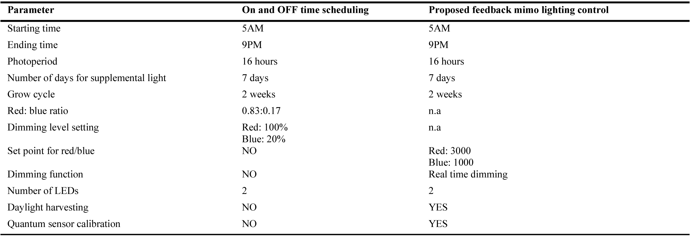
Table 1. Parameters of the comparison experiment for lighting control system performance.
The micro-green kale was selected as the test subject with a 2-week growth cycle. In the first week, the plants went from seeding to germination. The plant tray was covered fully by a cardboard to block the light. The cardboard was removed on the 1st day of the 2nd week and the plant tray was exposed to sunlight and supplemental LED light for one week before harvesting. Figure 11 shows the different stages of planting of the microgreen kale in which four plant trays were used for each set up. As shown in Fig. 12, microgreen kale, under the proposed lighting control system, grew as perfectly as the ones under the time scheduling scheme. However, slightly more even height and uniform density distribution were observed for the trays under the proposed lighting system than the ones under time scheduling system. The fresh weight of microgreen kale from all of the trays harvested at the end of the 2nd week are summarized in Table 2. The percent deviation shows the extent to which uniform light distribution can affect the growth. The fresh mass from trays under the ON-OFF time scheduling method (Tray #5, #6, #7, #8) had higher percent deviation than the trays under the proposed lighting control (Tray #1, #2, #3, #4). Particularly, Trays #7 and #8 show relatively high deviations, i.e., -27.4% and 29.1%, respectively. It is concluded that the weight distribution of all the four trays under the proposed lighting system had a more even fresh mass, compared to the fresh masses from the time scheduling lighting group. This proves the advantage of the proposed lighting system in providing a uniform light distribution on the plant surface during the daytime that sunlight varies from sunrise to sunset.
Figure 11
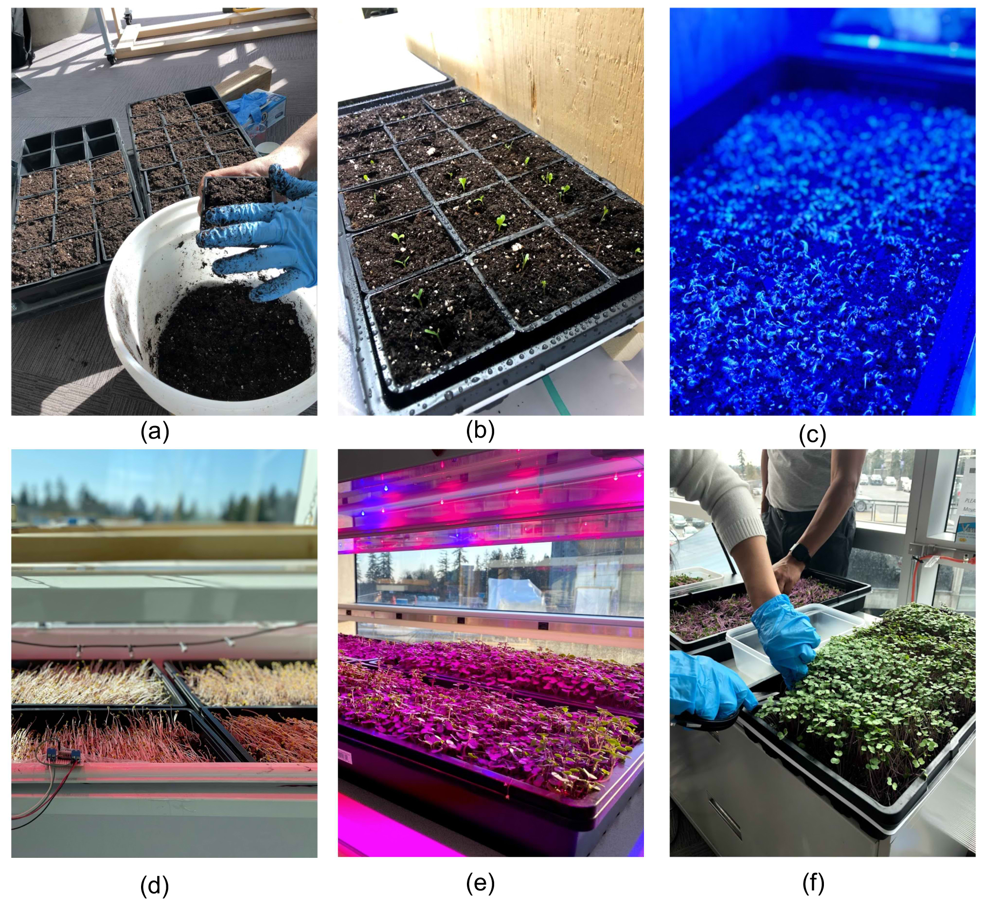
Fig. 11.Stages of planting the kale microgreen: (a) sowing, (b) germination, (c) LED complete dimming, (d) LED no dimming, (e) LED partial dimming and (f) plant harvesting.
Figure 12
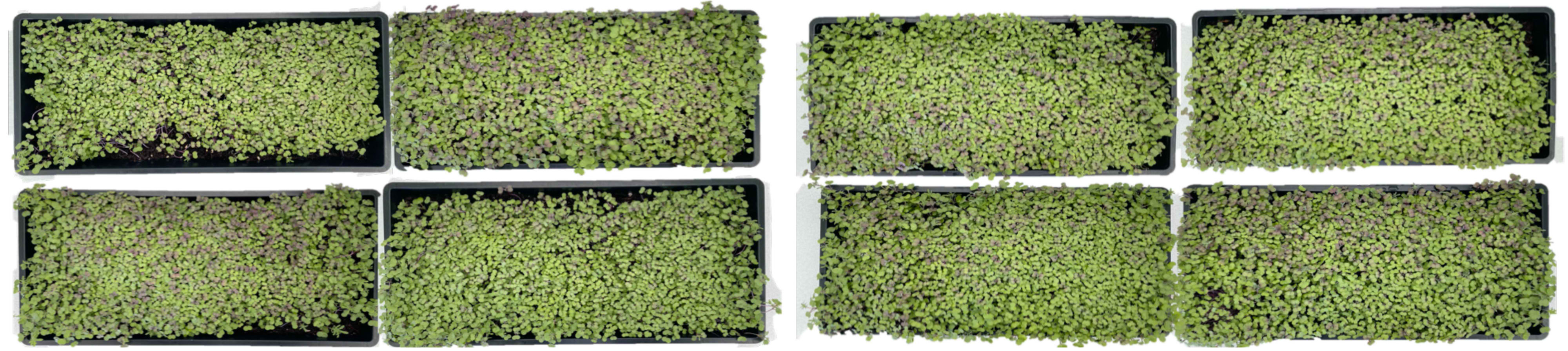
Fig. 12.Top view of the microgreen kale in plant trays: (a) time scheduling lighting system and (b) proposed feedback lighting control system.
Table 2

Table 2. Comparison of the effect on plant growth performance.
Under the proposed lighting control, red and blue channels on LEDs were automatically dimmed to harvest the daylight. The energy saving of the LED units were recorded during the 2nd week as shown in Fig. 13 and summarized in Table 3. For the specific light recipe given to the microgreen kale, we achieved an average 18.16% energy savings using the supplemental lighting during the grow cycle, while maintaining the plant productivity comparable to the conventional time scheduling lighting system.
Figure 13
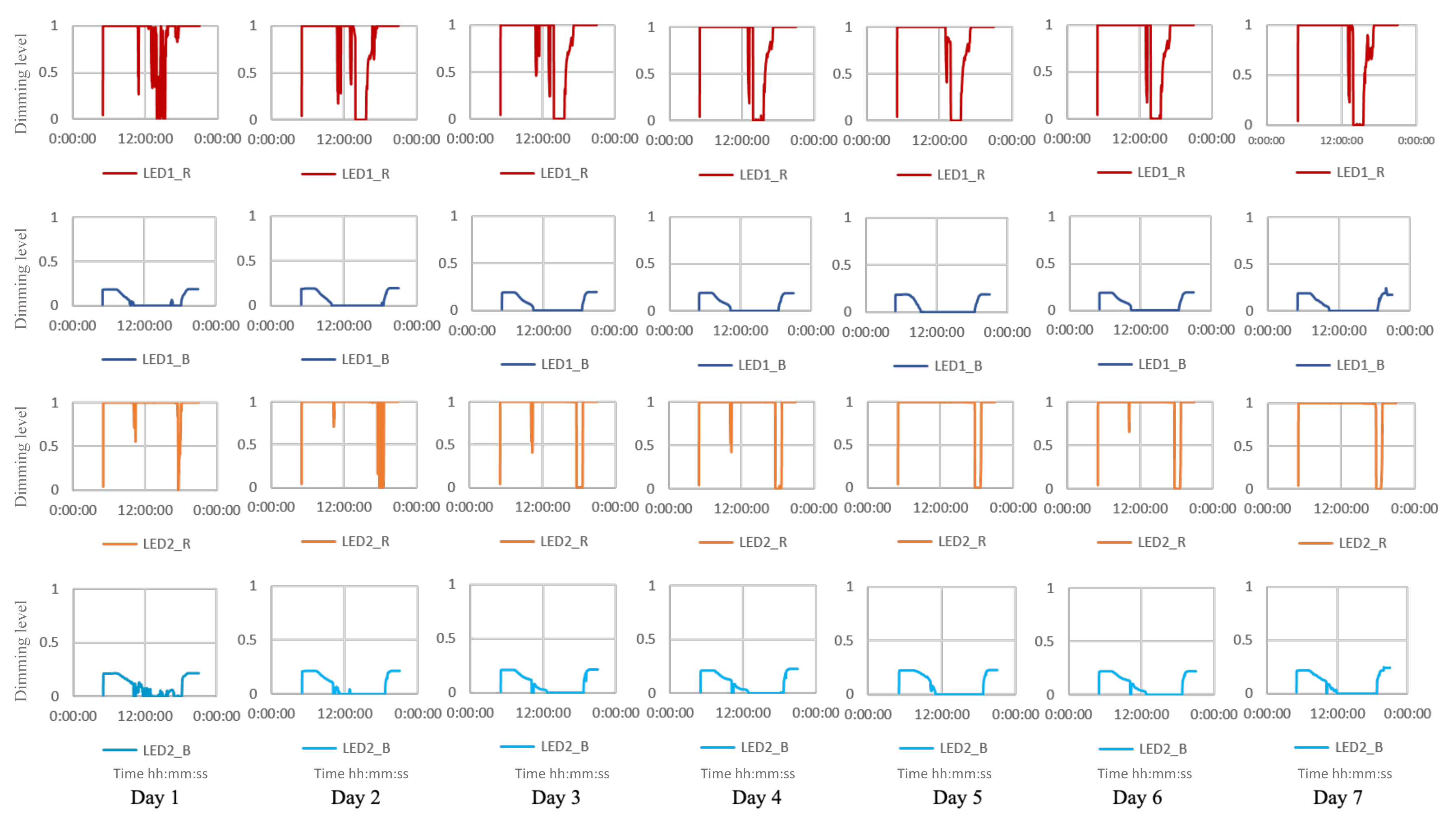
Fig. 13.Overview of the energy saving on red and blue channels of LEDs with running the proposed lighting system over one week.
Table 3
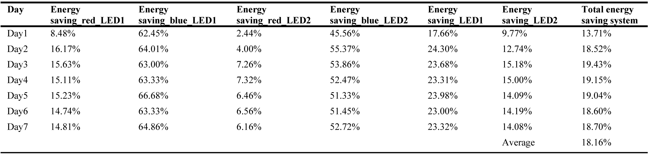
Table 3. Summary of energy saved by proposed lighting system set.
5. Conclusion
An IoT-enabled control and monitoring system with a built-in daylight harvesting control algorithm was presented in this paper. The experimental results and the system performance under two different sunlight conditions show that the system were analyzed. The compensation from the supplemental LEDs, specifically on red and blue channels, varied because of the daylight variations. The controller collected sensor data as the feedback signal provided and adjusted the dimming levels of LEDs for utilization in the daylight harvesting algorithm. Since over-saturation occurs, the system would expect that the LEDs are fully dimmed off to save the energy cost while the light requirement are still achieved. In the experiments conducted, we achieved 34% and 21% energy savings for sunny and cloudy days, respectively, when the proposed lighting system was compared with a conventional ON-OFF scheme. Also, the system achieved uniform lighting distribution and stable light output. Additionally, the live plant experiments conducted in this study has shown that the tested microgreen grew with more even height and uniform density, while being able to achieve the targeted DLI requirement.
Contributions
J. Jiang conducted the research, experiments and drafted the paper manuscript. M. Moallem primarily supervised the research, revised the manuscript. Y. Zheng co-supervised the research, provide suggestions and revised the manuscript.
Declaration of competing interest
The authors report no conflicting interests regarding this article. The authors are solely responsible for the content therein.
References
- I. Chew, D. Karunatilaka, CP. Tan, Smart Lighting: The Way Forward Reviewing the Past to Shape the Future, Energy and Buildings (2017) 180-191. https://doi.org/10.1016/j.enbuild.2017.04.083
- Y.J. Wen, A.M Agogino, Control of Wireless-Networked Lighting in Open-Plan Offices, Light Res Technol 43 (2011) 235–248. https://doi.org/10.1177/1477153510382954
- W. Li, L. Zhujun, Z. Chunfeng, Research and application of the fuzzy control used in the wireless illumination measurement and control system of the greenhouse. In: Proceedings of the 2011 Chinese Control and Decision Conference, 2011, pp. 1363–1367. https://doi.org/10.1109/ccdc.2011.5968402
- A. Peña-García, F. Salata, The Perspective of Total Lighting as A Key Factor to Increase the Sustainability of Strategic Activities, Sustain 12 (2020) 2751. https://doi.org/10.3390/su12072751
- T. Penev, V. Radev, Effect of Lighting on the Growth, Development, Behaviour, Production and Reproduction Traits in Dairy Cows, Int J Curr Microbiol Appl Sci (2014) 798–810. https://doi.org/10.1016/j.solener.2013.06.016
- R.R Peters, L.T Chapin, K.B Leining, et al, Supplemental Lighting Stimulates Growth and Lactation in Cattle, Science (1978) 911–912. https://doi.org/10.1126/science.622576
- N. Taylor, N. Prescott, G. Perry, et al, Preference of Growing Pigs for Illuminance, Appl Anim Behav Sci (2006) 19–31.
- J.C. Huth, G.S Archer, Comparison of Two LED Light Bulbs to A Dimmable CFL And Their Effects on Broiler Chicken Growth, Stress, And Fear, Poult Sci (2015) 2027–2036. https://doi.org/10.3382/ps/pev215
- P. Garcia-Caparros, R.M Chica, E.M Almansa, et al, Comparisons of Different Lighting Systems for Horticultural Seedling Production Aimed at Energy Saving, Sustain 10 (2018) 3351. https://doi.org/10.3390/su10093351
- P. García-Caparrós, E.M Almansa, R.M Chica, et al, Effects of Artificial Light Treatments on Growth, Mineral Composition, Physiology, And Pigment Concentration in Dieffenbachia Maculata Compacta Plants, Sustain 11 (2019) 2867. https://doi.org/10.3390/su11102867
- J.K Craver, J.K Boldt, R.G Lopez, Comparison of Supplemental Lighting Provided by High-Pressure Sodium Lamps or Light-Emitting Diodes for The Propagation and Finishing of Bedding Plants in A Commercial Greenhouse, HortScience 54 (2019) 52–59. https://doi.org/10.21273/hortsci13471-18
- A. Vadiee, V. Martin, Energy Management Strategies for Commercial Greenhouses, Appl Energy 114 (2014) 880–888. https://doi.org/10.1016/j.apenergy.2013.08.089
- B. Roisin, M. Bodart, A. Deneyer, et al, Lighting Energy Savings in Offices Using Different Control Systems and Their Real Consumption, Energy Build 40 (2008) 514-523. https://doi.org/10.1016/j.enbuild.2007.04.006
- Yeh LW, Lu CY, Kou CW, et al, Autonomous Light Control by Wireless Sensor and Actuator Networks, IEEE Sens J. 10 (2010) 1029-1041. https://doi.org/10.1109/JSEN.2010.2042442
- X. Qu, S.C Wong, C.K Tse, Temperature Measurement Technique for Stabilizing the Light Output of RGB LED Lamps. IEEE Trans Instrum Meas 59 (2010) 661–670. https://doi.org/10.1109/tim.2009.2025983
- J. Craver, J. Gerovac, D. Kopsell, et al, Comparison of Light Qualities and DLI For Sole‐Source Lighting of Microgreens and Bedding Plant Plugs, Purdue Floriculture (2015).
- D. Llewellyn, K. Schiestel, Y. Zheng, Light-Emitting Diodes Can Replace High-Pressure Sodium Lighting for Cut Gerbera Production, HortScience 54 (2019) 95–99. https://doi.org/10.21273/hortsci13270-18
- T. Namgyel, C. Khunarak, S. Siyang, et al, Effects of supplementary LED light on the growth of lettuce in a smart hydroponic system, In: 2018 10th International Conference on Knowledge and Smart Technology: Cybernetics in the Next Decades, KST 2018. Institute of Electrical and Electronics Engineers Inc., 2018, pp. 216–220. https://doi.org/10.1109/kst.2018.8426202
- Y. Kong, Y. Zheng, Variation of Phenotypic Responses to Lighting Using A Combination of Red and Blue Light-Emitting Diodes Versus Darkness in Seedlings Of 18 Vegetable Genotypes, Can J Plant Sci 99 (2019) 159–172. https://doi.org/10.1139/cjps-2018-0181
- J. Muangprathub, N. Boonnam, S. Kajornkasirat, et al, Iot And Agriculture Data Analysis for Smart Farm, Comput Electron Agric 156 (2019) 467–474. https://doi.org/10.1016/j.compag.2018.12.011
- A.N Harun, N. Mohamed, R. Ahmad, et al, Improved Internet of Things (Iot) Monitoring System for Growth Optimization of Brassica Chinensis, Comput Electron Agric 164 (2019).
- G. Mois, S. Folea, T. Sanislav, Analysis of Three IoT-Based Wireless Sensors for Environmental Monitoring, IEEE Trans Instrum Meas 66 (2017) 2056–2064. https://doi.org/10.1109/tim.2017.2677619
- CC. Mpelkas, Light Sources for Horticultural Lighting, IEEE Trans Ind Appl 16 (1980) 557–565. https://doi.org/10.1109/tia.1980.4503829
- W. Qiu, L. Dong, F. Wang, et al, Design of Intelligent Greenhouse Environment Monitoring System Based on Zigbee And Embedded Technology, In: Proceedings of 2014 IEEE International Conference on Consumer Electronics - China, ICCE-C 2014. Institute of Electrical and Electronics Engineers Inc., 2015. https://doi.org/10.1109/icce-china.2014.7029857
- D. Feliciano Cayanan, M. Dixon, Y. Zheng, Development of An Automated Irrigation System Using Wireless Technology and Root Zone Environment Sensors, Acta Hortic 797 (2008) 167–172. https://doi.org/10.17660/actahortic.2008.797.22
- L.D Albright, A.J Both, A.J. Chiu, Controlling Greenhouse Light to A Consistent Daily Integral, ASAE American Soc Agric Eng 43 (2000) 421–431. https://doi.org/10.13031/2013.2721
- A. Yano, K. Fujiwara, Plant Lighting System with Five Wavelength-Band Light-Emitting Diodes Providing Photon Flux Density and Mixing Ratio Control, Plant Methods 8 (2012). https://doi.org/10.1186/1746-4811-8-46
- D. Caicedo, A. Pandharipande, Distributed Illumination Control with Local Sensing and Actuation in Networked Lighting Systems, IEEE Sens J 13 (2013) 1092–1104. https://doi.org/10.1109/jsen.2012.2228850
- A.N. Harun, Ani NN, R. Ahmad, et al, Red and blue LED with pulse lighting control treatment for brassica chinensis in indoor farming, In: 2013 IEEE Conference on Open Systems, ICOS 2013. IEEE, pp. 231–236. https://doi.org/10.1109/icos.2013.6735080
- Y. Kong, D. Llewellyn, Y. Zheng, Response of Growth, Yield, And Quality of Pea Shoots to Supplemental Light-Emitting Diode Lighting During Winter Greenhouse Production, Can J Plant Sci 98 (2017) 732–740. https://doi.org/10.1139/cjps-2017-0276
- T. Schwend, M. Beck, D. Prucker, et al, Test of A PAR Sensor-Based, Dynamic Regulation of LED Lighting in Greenhouse Cultivation of Helianthus Annuus, Eur J Hortic Sci 81 (2016) 152–156.
- I. Seginer, L.D. Albright, I. Ioslovich, Improved Strategy for A Constant Daily Light Integral in Greenhouses, Biosyst Eng 93 (2006) 69–80. https://doi.org/10.1016/j.biosystemseng.2005.09.007
- K.H. Kjaer, C.O Ottosen, B.N. Jørgensen, Cost-Efficient Light Control for Production of Two Campanula Species, Sci Hortic (Amsterdam) 129 (2011) 825–831. https://doi.org/10.1016/j.scienta.2011.05.003
- D. Singh, C. Basu, M. Meinhardt-Wollweber, et al, LEDs For Energy Efficient Greenhouse Lighting, Renew Sustain Energy Rev 49 (2015) 139–147. https://doi.org/10.1016/j.rser.2015.04.117
- RC. Morrow, LED lighting in horticulture, In: HortScience. 2008, pp. 1947–1950. https://doi.org/10.1016/j.solener.2013.06.016
- J. Jiang, M. Moallem, Development of Greenhouse LED System with Redlblue Mixing Ratio and Daylight Control, In: 2018 IEEE Conference on Control Technology and Applications, CCTA 2018, 2018, pp. 1197–1202, Denmark. https://doi.org/10.1109/ccta.2018.8511374
- S.Y. Hui, Y.X. Qin, A General Photo-Electro-Thermal Theory for Light Emitting Diode (LED) Systems, IEEE Trans Power Electron 24 (2009) 1967–1976. https://doi.org/10.1109/tpel.2009.2018100
- Y.X. Qin, S.Y. Hui, Comparative study on the structural designs of led devices & systems based on the general photo-electro-thermal theory. In: 2009 IEEE Energy Conversion Congress and Exposition, ECCE 2009. IEEE Computer Society, 2009, pp. 2833–2839. https://doi.org/10.1109/ecce.2009.5316478
- X. Tao, S.Y. Hui, Dynamic Photoelectrothermal Theory for Light-Emitting Diode Systems. IEEE Trans Ind Electron 59 (2012) 1751–1759. https://doi.org/10.1109/tie.2011.2109341
- J. Jiang, A. Mohagheghi, M. Moallem, Energy-Efficient Supplemental LED Lighting Control for A Proof-Of-Concept Greenhouse System, IEEE Trans Ind Electron 67 (2020) 3033–3042. https://doi.org/10.1109/tie.2019.2912762
- R. Dangol, T. Kruisselbrink, A. Rosemann, Effect of Window Glazing on Colour Quality of Transmitted Daylight, Journal of Daylighting 4 (2017) 37-47. https://dx.doi.org/10.15627/jd.2017.6
- L. Doulos, A. Tsangrassoulis, V. Topalis, The Role of Spectral Response of Photosensors In Daylight Responsive Systems, Energy Build 40 (2008) 588–599. https://doi.org/10.1016/j.enbuild.2007.04.010
- A.P. Torres, R.G. Lopez, Commercial Greenhouse Production - Measuring Daily Light Integral in A Greenhouse, https://www.extension.purdue.edu/extmedia/ho/ho-238-w.pdf.
- MechaTronix, MechaTronix Horticulture Lighting, Typical PPFD and DLI values per crop, https://www.horti-growlight.com/typical-ppfd-dli-values-per-crop.
Copyright © 2021 The Author(s). Published by solarlits.com.

3306
Total views
Citations
SHARE ON


