Optimization of Daylighting Design Using Self-Shading Mechanism in Tropical School Classrooms with Bilateral Openings

^a Engineering Physics Doctorate Program, Department of Engineering Physics, Faculty of Industrial Technology Institut Teknologi Bandung, Jl. Ganesha 10, Labtek VI, Bandung 40132, Indonesia
^b Architecture Program, Faculty of Engineering, Universitas Malikussaleh, Jl. Cot Teungku Nie, Aceh Utara 24355, Indonesia
^c Building Physics Research Group, Department of Engineering Physics, Faculty of Industrial Technology, Institut Teknologi Bandung, Jl. Ganesha 10, Labtek VI, Bandung 40132, Indonesia
^d Building Technology Research Group, Department of Architecture, School of Architecture, Planning, and Policy Development, Institut Teknologi Bandung, Jl. Ganesha 10, Labtek VI, Bandung 40132, Indonesia
^e Unit Building Physics and Services, Department of the Built Environment, Eindhoven University of Technology, PO Box 513, 5600 MB Eindhoven, the Netherlands
^f Advanced Functional Material Research Group, Department of Engineering Physics, Faculty of Industrial Technology, Institut Teknologi Bandung, Jl. Ganesha 10, Labtek VI, Bandung 40132, Indonesia

*Corresponding author.
atthaillah@unimal.ac.id (Atthaillah)
armanto@tf.itb.ac.id (R. A. Mangkuto)
donny@ar.itb.ac.id (M. D. Koerniawan)
j.hensen@tue.nl (J. L.M. Hensen)
brian@tf.itb.ac.id (B. Yuliarto)

History: Received 15 April 2022 | Revised 1 July 2022 | Accepted 9 July 2022 | Published online 13 August 2022

Citation: Atthaillah, Rizki A. Mangkuto, M. Donny Koerniawan, Jan L.M. Hensen, Brian Yuliarto, Optimization of Daylighting Design Using Self-Shading Mechanism in Tropical School Classrooms with Bilateral Openings, Journal of Daylighting 9 (2022) 117-136. https://dx.doi.org/10.15627/jd.2022.10

Figures and tables

Abstract

Despite its potential, daylighting strategies in school classrooms in the tropical climate regions is little explored in the literature. The use of two-sided or bilateral daylight opening, as well as the self-shading mechanism using sloped walls, are currently seen as potential strategies to achieve good daylighting in tropical buildings. This study thus aims at exploring and optimizing self-shading design possibilities for creating daylight-friendly, tropical elementary school classrooms with bilateral openings, by means of sensitivity and uncertainty analyses. Design parameters such as façade orientation, window-to-wall ratio, window elevations, wall slopes, interior surface reflectance and glazing transmittance are considered in the model of a hypothetical, typical classroom without shading devices. Climate-based daylight metrics such as UDI_{250-750 lx}, sDA_300/50% and ASE_1000,250 are utilized as the performance indicators. Computational modelling with Honeybee [+] in Rhinoceros/ Grasshopper platform is employed to conduct the annual daylight simulation. Multi-objective optimizations using genetic algorithms (GA) through Octopus with SPEA-2 algorithms are performed to determine the optimum design solutions following the sensitivity and uncertainty analysis. The slope and WWR of the wall that faces west, southwest, south, or southeast, has the strongest influence on the defined objective function that includes all daylight metrics. To achieve the optimum daylight performance, design of the opposing window façades of school classrooms with bilateral openings should not be identical.

Keywords

Daylighting, Bilateral opening, Tropical climate, Climate-based daylight metric

1. Introduction

Daylighting in school classrooms is known to be beneficial for improving students’ wellbeing and performance, while reducing electrical energy consumption in the building. Those benefits have been acknowledged by many researchers across the globe [1–8]. However, despite its potential, investigation on daylighting strategies in school classrooms in the tropical climate regions, where daylight is abundantly available, is less popular than that in the non-tropical regions [9–11].

With regards to daylighting strategies, in general, some studies have investigated the utilization of shading devices [9,11–18], light shaft [19–21], smart envelope [13,22–27], curve façade [28] and toplighting [2,29–31] strategies. Majority of those studies examine daylight design strategies on the one-sided daylight apertures, also known as the unilateral opening typology. In some cases, the unilateral opening may be combined with toplighting in school classrooms [30].

Moreover, most of the studies also explore the optimum design for the shading parameters alone, without interaction with other design input variables. Few studies have attempted examining multiple input design variables for achieving the optimum daylight performance [32,19,33]. Also, the unilateral opening typology is typically considered since most of the studies assumes similarity with office spaces utilization, in which the use of shading or glare control devices is mandatory. Meanwhile, self-shading strategies, for instance by constructing sloped walls, to achieve optimum daylight performance is rather limited [2] for the hot-arid climate. Some of the most relevant daylighting studies worldwide, focusing on the classroom, are summarized in Table 1, organized by the publication date.

Table 1

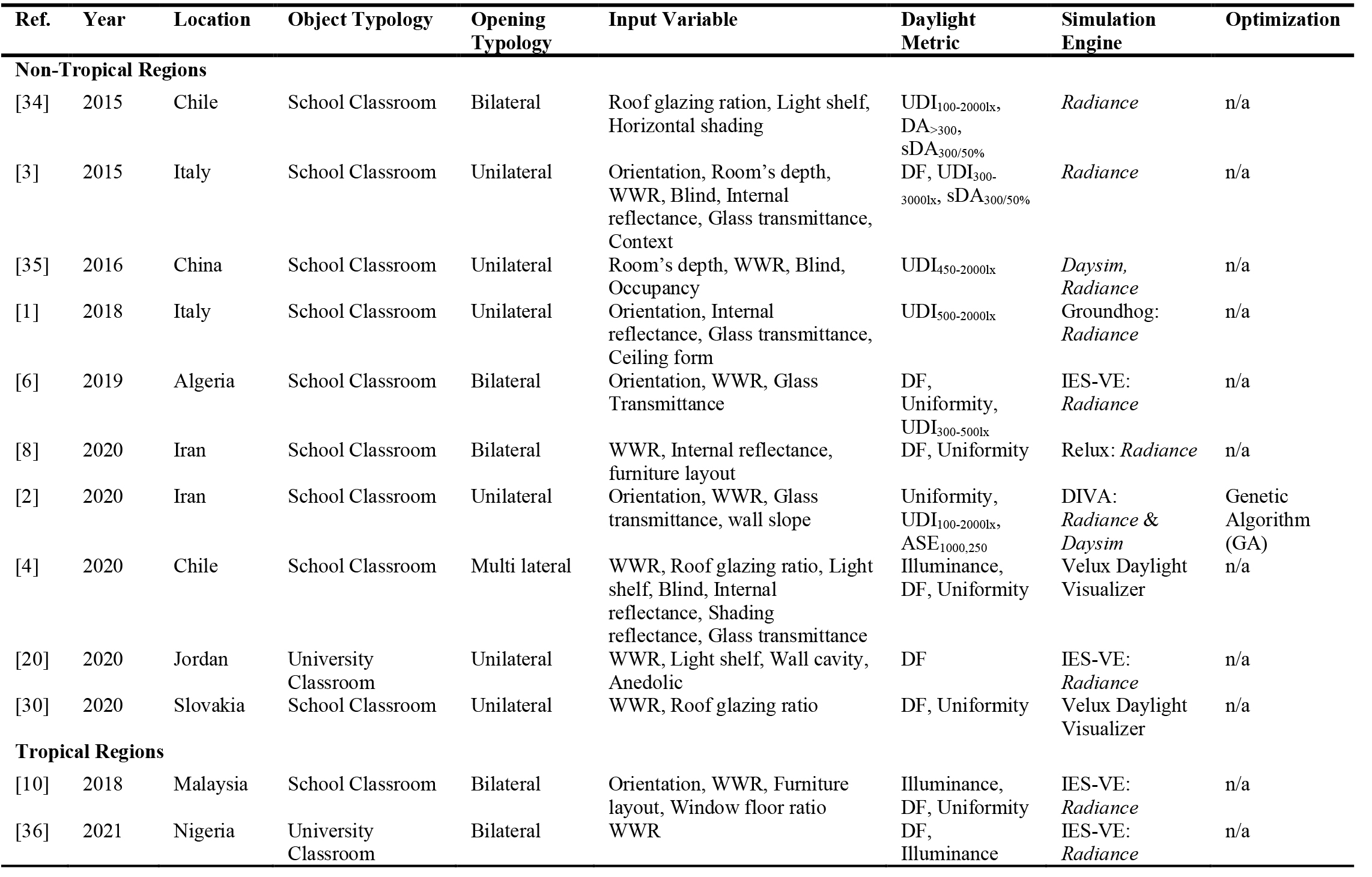
Daylighting studies at school or university classroom utilizing simulation method in the non-tropical and tropical climate regions (excluding Indonesia as the case study).

Table 1. Daylighting studies at school or university classroom utilizing simulation method in the non-tropical and tropical climate regions (excluding Indonesia as the case study).

As shown in Table 1, 60% of the daylighting studies in non-tropical regions focus on unilateral opening typology. Meanwhile, most daylighting studies in the tropics focus on bilateral opening typology, as in the case of Malaysia and Nigeria. The utilization of bilateral openings in the tropics is due to the advantage of cross ventilation, which can also be beneficial from daylighting perspective.

Regarding the daylight metrics, static metric such as daylight factor (DF) is still utilized mostly in the tropics due to relatively small seasonal variation. Meanwhile, various dynamic daylight metrics, which incorporate local weather files, are widely utilized in the non-tropical regions. Furthermore, most daylighting studies on classrooms are mainly conducted using simulation without implementing an optimization method such as a genetic algorithm (GA), except Reference [2], which was conducted in hot arid climates. GA optimization is required particularly if the complexity of the input and output variables are increased, so that brute force simulation methods become ineffective.

In Indonesia, which is one of the tropical countries with a population of more than 270 million, daylighting studies in school classrooms are limited to some major cities such as Makassar and Surabaya [37,38]. The current practice of designing school classrooms, particularly the state-funded ones, in Indonesia is mostly based on typicality, guided by national or local regulations which mainly focus solely on the geometrical size and features of the classrooms [39]. This regulation typically assumes similar types of microclimates throughout the country and does not involve technical requirements of daylight within the space. Therefore, Indonesian classroom designs are mostly identical in geometry (Fig. 1) and are not necessarily daylight-friendly, despite the relatively high amount of daylight availability in the region. This situation may lead to less-than-optimum design practice of daylighting in schools across the country.

Figure 1

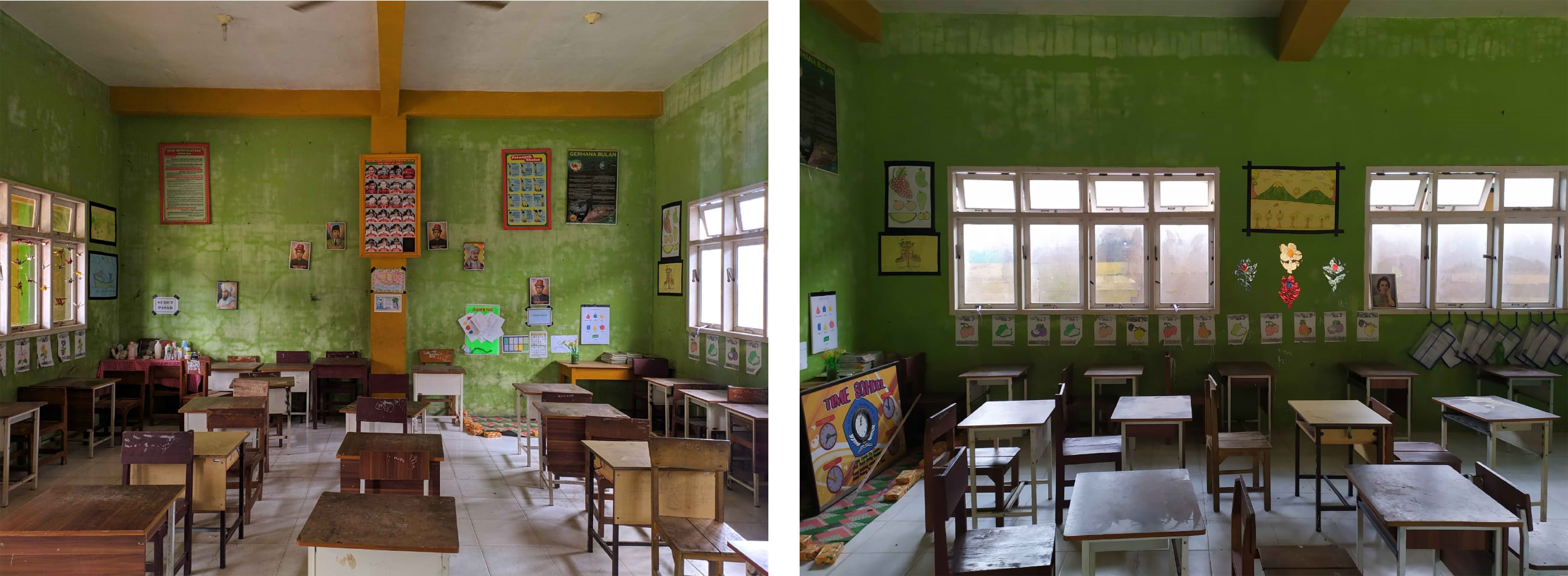
Fig. 1. Interior view of a typical, state-funded elementary school classroom in Indonesia.

Several recent studies have suggested that most Indonesian classrooms receive insufficient amount of daylight [37,40,41]. This situation consequently contributes to a higher amount of electrical energy consumption due to the unnecessary use of electric lighting and/or air-conditioning. The lack of sufficient daylight inside the classroom can also be associated to the students’ poor performance and alertness [2,7,9,42,43]. In the end, schools with such classrooms become ineffective in delivering their educational purpose to the students.

Meanwhile, design of state-funded school classrooms in Indonesia is regulated by the Ministry of Education and Culture [39], which recommends the use of two-sided daylight apertures, also known as the bilateral opening typology (Fig. 1). Assessment on the optimum massing strategies in daylighting design for such opening typology is nonetheless still missing. Furthermore, it is argued that the self-shading mechanism can be seen as one of the features in defining good daylighting inside buildings in the tropical climate, as is the case in the hot arid climate [2]. In addition, the self-shading mechanism shall improve the architectural outlook of school classrooms, through variation of the façade slope, as opposed to the typically uniform design. Therefore, this study attempts to fill the gap.

Having described the motivation, this study aims at exploring and optimizing self-shading design possibilities to create daylight-friendly, tropical school classrooms with bilateral openings on the opposing façades, with the case study of Indonesia. The novelty of this study is thus the proposed building massing strategy to accommodate the self-shading design feature in daylit rooms with bilateral opening, which are rarely discussed in literature.

The daylighting design in this study are attributed to the façade design variables, such as window elevation, window-to-wall ratio (WWR), wall slopes, internal reflection and glazing transmittance as suggested in Table 1 for external façade design. Also, design solutions are investigated using GA optimization due to the complexity of the input variables. Sensitivity analysis is conducted as the initial step to propose the design guideline in achieving daylight-friendly school classrooms, following multi-objective optimization regarding the relevant climate-based metrics.

The paper is organized as follows. Section 2 describes the methods. Sections 3 and 4 provide the results and discussion, whereas Section 5 concludes the paper. Figure 2 demonstrates in detail the complete structure of this work.

Figure 2

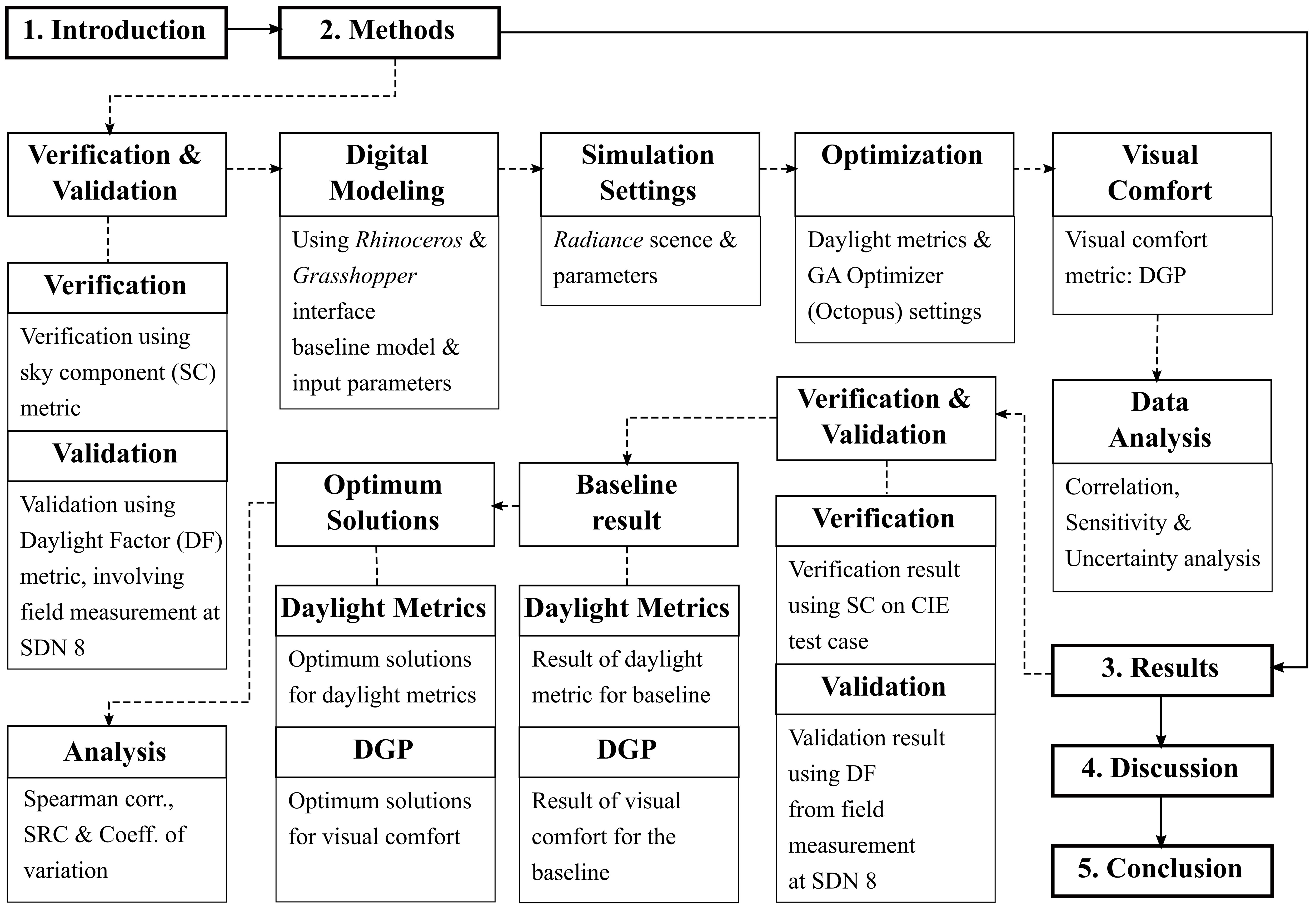
Fig. 2. Workflow of this study; solid lines represent the section flow, while dash lines represent the subsection flow.

2. Methods

This study employs computational simulation since it implements the annual daylight metrics as the performance criteria. As shown in Table 1, most daylighting studies in the literature have utilized Radiance. Also, Radiance has undergone short-term [9], long-term [44,45] and various scenes complexities [46–48] validation, all of which conclude that it is indeed a valid daylight simulation engine. Nevertheless, this study conducts the verification and validation to determine the appropriate simulation setting of Radiance parameters, in order to minimize the simulation result discrepancy. Next, this study conducts design optimization using GA. Furthermore, various tools utilized in this study are depicted in Fig. 2.

2.1. Verification and Validation

2.1.1. Verification

Analytical verification is conducted to find the reliable Radiance parameters for simulating the sky component (SC) in the modelled room. The SC is calculated based on assumption that the interior and exterior surfaces have no reflection, no window glass and no surrounding context [49]. Based on these assumptions, verification is focused on the simulation engine settings. The SC is calculated under the standard CIE overcast sky condition [50].

Furthermore, this study utilizes the CIE test case 5.13 [51] to define the SC calculation points inside the modelled, hypothetical space as illustrated in Fig. 3. Also, verification is conducted based on the default low, medium and high settings in Honeybee [+] interface (Table 2).

Figure 3

Fig. 3. Interior perspective of the hypothetical room in the CIE test case 5.13 [51].

Table 2

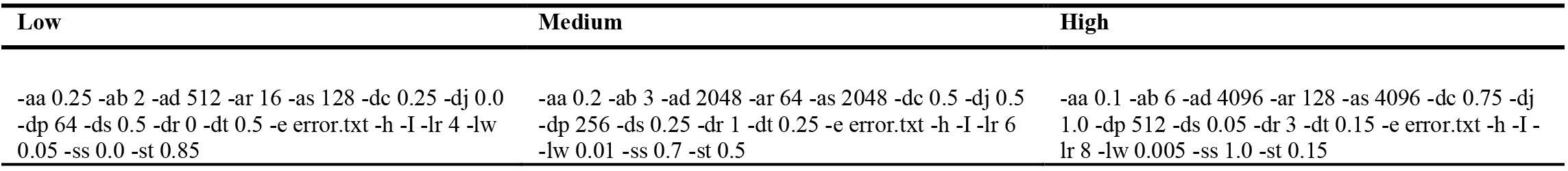
Table 2. Radiance setting for verification against the SC simulation in this study.

The simulated SC values on each calculation point in each setting are thus compared with the analytical values to obtain the relative error ε [52,53], as defined in Eq. (1).

\[ \varepsilon=\frac{\left|SC_{simulation}-SC_{analytical}\right|}{SC_{analytical}}\times100\% \]

2.1.2. Validation

A field measurement was also performed to validate the simulation setting, by integrating the room surface reflectance and the glass transmittance from an existing classroom in SDN 8 Banda Sakti Lhokseumawe, Indonesia, hereinafter referred to as called as SDN 8. The measurement was conducted on 16-20 November 2020 and 23-27 November 2020, using Krisbow KW0600291 illuminance meter (error ± 0.01 lx). Six measurement points were located inside the classroom and the position were as instructed by the Indonesian national standard [54] at elevation of 0.75 m (Fig. 4). An external point outside the classroom was also measured at elevation of 0.50 m, which was set to block the direct sunlight, as to model the overcast sky condition. At each sensor point, the measurement was conducted at 8:00, 10:00, 12:00, 14:00 and 16:00 local time. Furthermore, the room surface reflectance (ρ_s), assuming a Lambertian surface, is estimated by dividing the reflected exitance (M_ρ,s) to the illuminance received on each surface (E_s) [55], so that:

\[ \rho_s=\frac{M_{\rho,s}}{E_s} \]

The surface reflectance for floor (ρ_f), wall (ρ_w), ceiling (ρ_c), glass transmittance (τ) and external object reflectance (ρ_ctx) from the field measurement is tabulated in Table 3. The glass transmittance is based on the product installed for the window glass (Asahimas Indoflot 3mm) with the original τ = 0.89. Due to the relatively low maintenance of the glazing, the transmittance value in this work is reduced to 0.7. Since there is a perimeter building next to the classroom, the external surface reflectance is also measured using Eq. (2). The external surface reflectance value is later used for the material setting in the simulation. Furthermore, the geometrical model of the classroom and the entire building of SDN 8 is depicted in Fig. 5.

Table 3

Table 3. The existing surface reflectance and transmittance values in typical classrooms in SDN 8.

Figure 4

Fig. 4. Plan view of the illuminance sensor points in the field measurement.

Figure 5

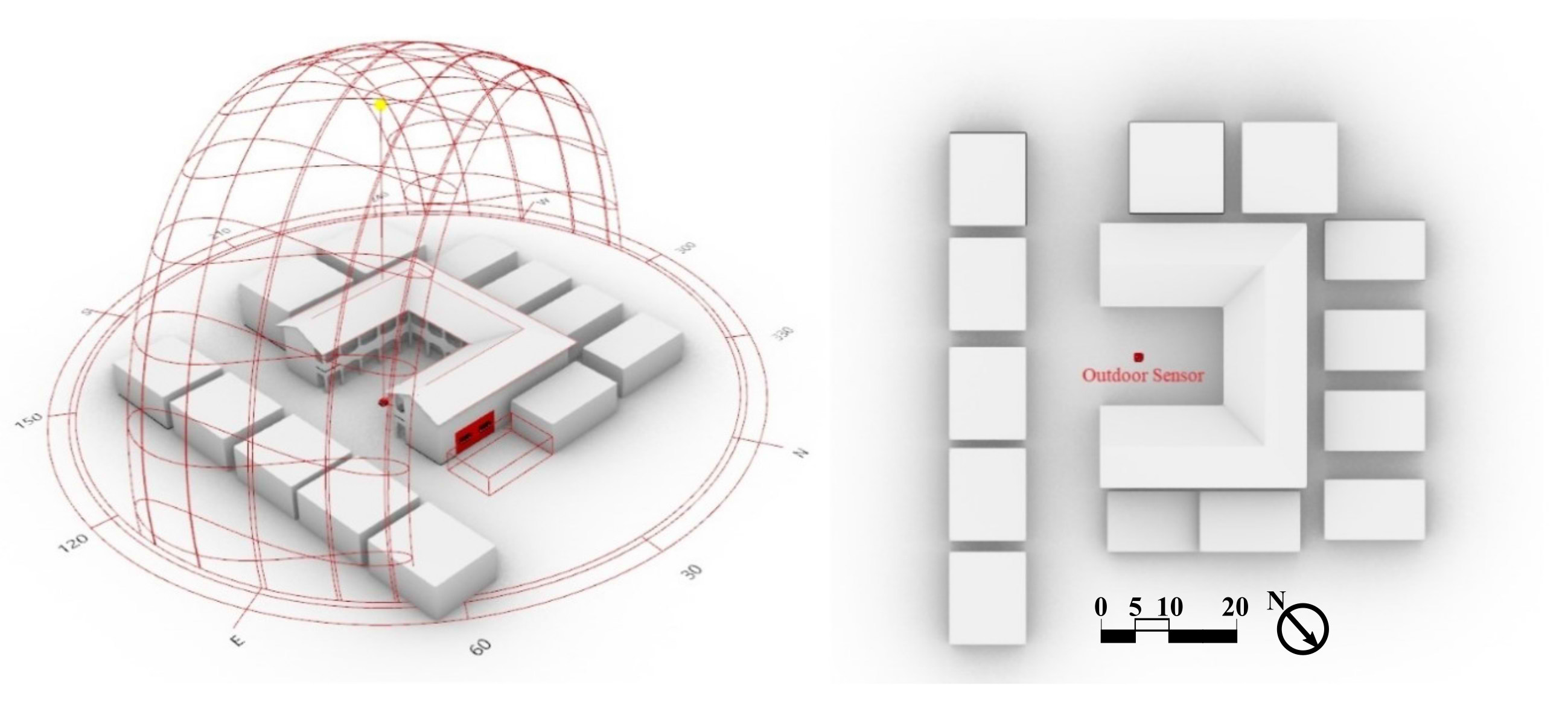
Fig. 5. (a) Perspective and (b) siteplan of the geometrical model of SDN 8; scale bar is in meter.

For the field measurement in SDN 8, the daylight factor (DF) at each measurement hour is averaged. Similarly, the DF values are also computed based on the simulation of SDN 8. The DF values obtained from the field measurement are compared with the analytical values. The relative error ε [52,53] for each sensor point is thus defined in Eq. (3).

\[ \varepsilon=\frac{\left|DF_{simulation}-DF_{measurement}\right|}{DF_{measurement}}\times100\% \]

2.2. Digital model

Digital models of this study are constructed for two Indonesian cities, namely Bandung (6°54'14" S, 107°37'7" E, 675~1050 m above sea level) and Lhokseumawe (5°10'0" N, 97°8'0" E, 2~24 m above sea level). Note that while both cities are located in hot, humid climate regions, the former is located slightly at the south of the equator, while the latter is slightly at the north.

Furthermore, Bandung represents typical mountainous cities located at a high altitude, while Lhokseumawe represents typical coastal cities located at a low altitude, so both cities well represent the diversity in the tropical region. Figure 6 illustrates the climatic variation in terms of their total radiation and atmospheric condition throughout the year. Those are the main basis for selecting the two cities as the case studies in this work.

Figure 6

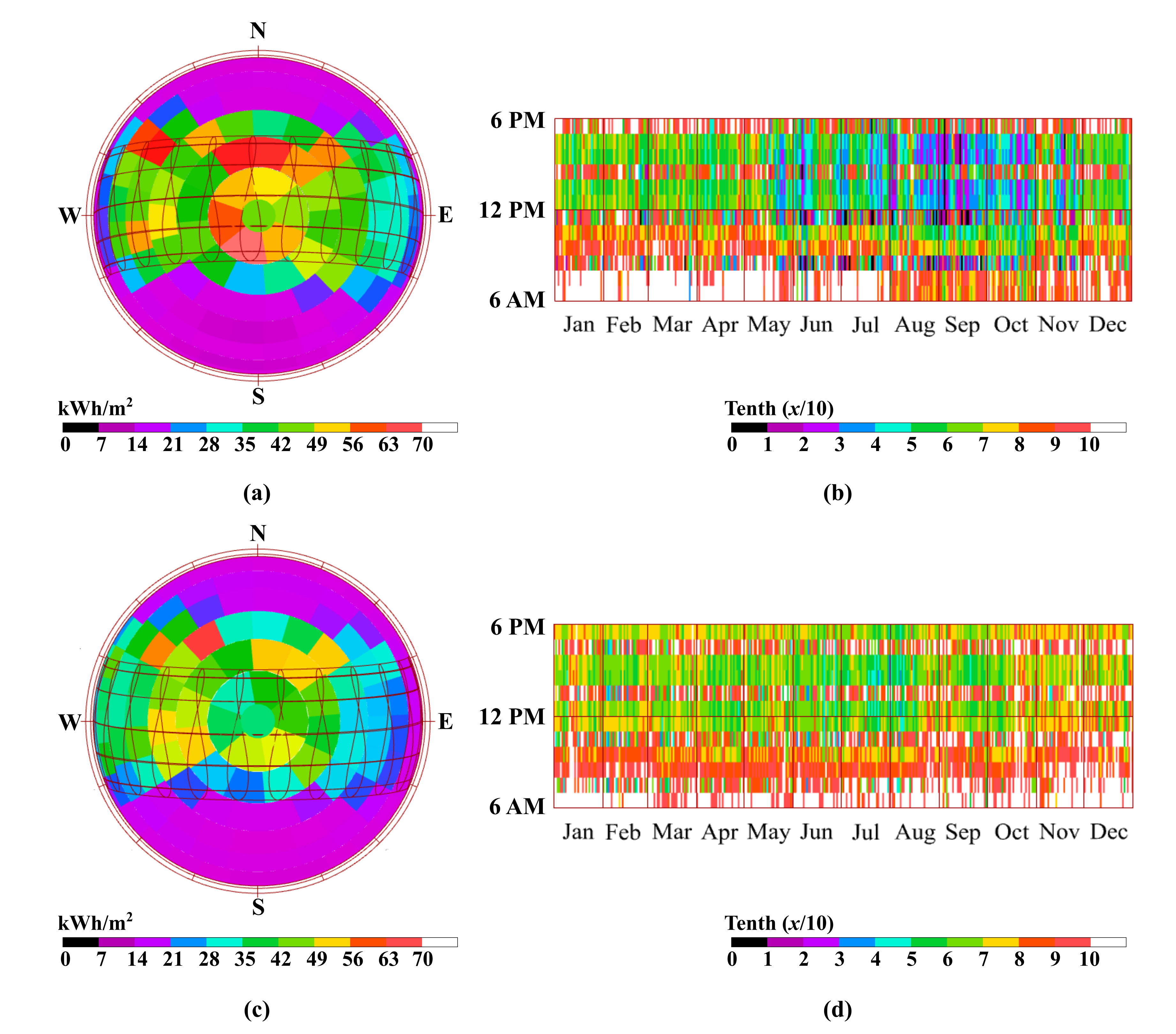
Sun path and total yearly radiation on the sky dome with 145 patches for (a) Bandung and (c) Lhokseumawe; and annual atmospheric conditions in terms of cloud coverage on 0~10 scale (0 for clear sky and 10 for full cloud coverage) in (b) Bandung and (d) Lhokseumawe.

Fig. 6. Sun path and total yearly radiation on the sky dome with 145 patches for (a) Bandung and (c) Lhokseumawe; and annual atmospheric conditions in terms of cloud coverage on 0~10 scale (0 for clear sky and 10 for full cloud coverage) in (b) Bandung and (d) Lhokseumawe.

For the case study, an isolated hypothetical school classroom with the internal size of 7.0 m × 8.0 m × 3.5 m with typical bilateral windows is considered. The internal size of the room refers to the Indonesian national regulation for elementary school classroom [39]. The room is modelled using Rhinoceros and Grasshopper platform [56,57], which is done for effortless integration of geometries in the optimization process during the later stage [58]. In this study, the building mass strategies are implemented for the cities of Bandung and Lhokseumawe in Indonesia. The involved input variables, or design parameters, are window elevation, WWR, wall slope, interior reflectance, and glass transmittance. Four cardinal orientations of the classroom building are considered, namely 0°, 45°, 90° and 135° (Fig. 7). All input variables with their respective symbols (X₁ until X₁₀), as well as the building orientations, are illustrated in Fig. 7.

Figure 7

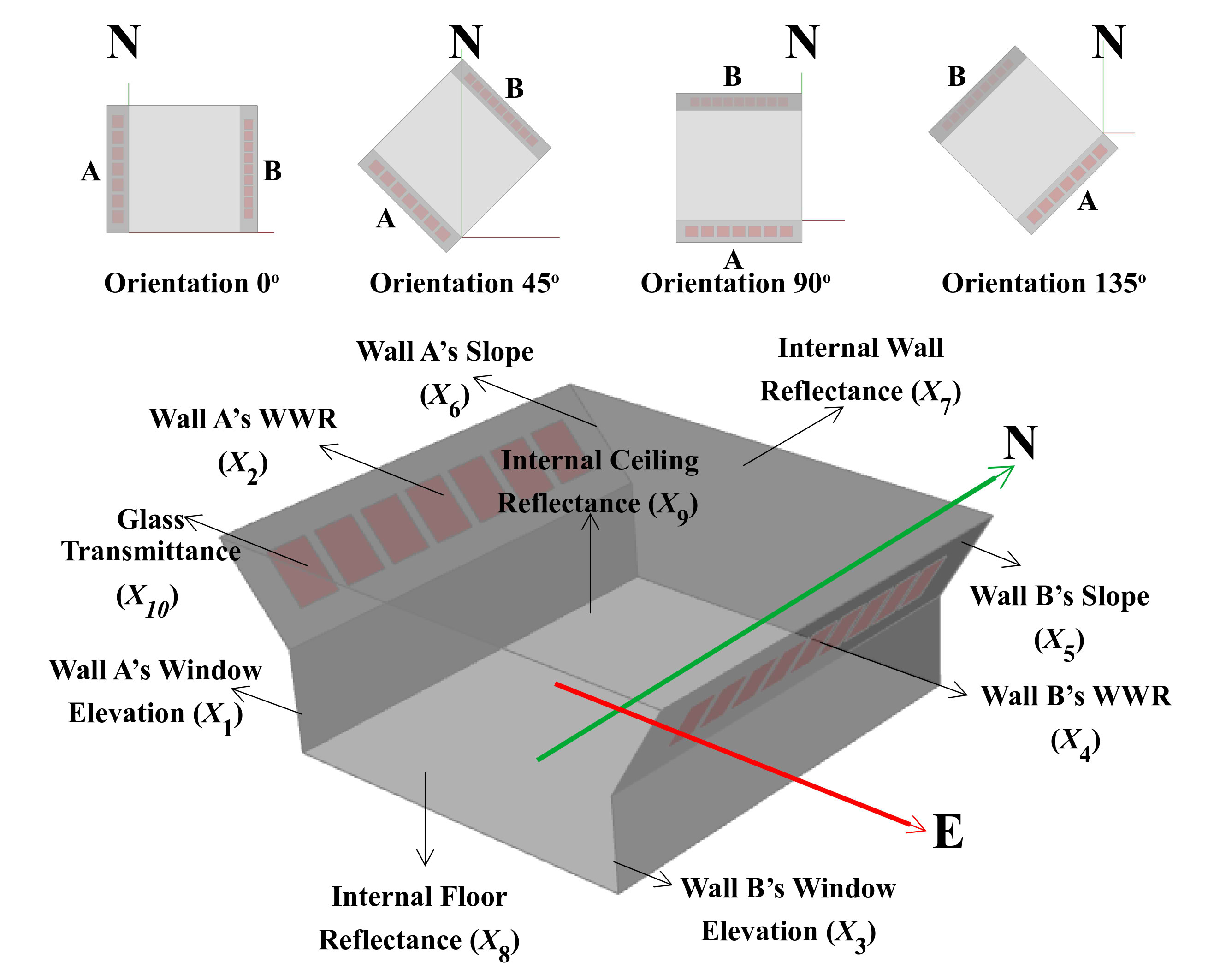
Fig. 7. Façade orientation of the modelled hypothetical classroom and description of the observed variables.

The material properties of the room are defined within certain ranges, to prepare the model for optimization process in the later stage. For the walls, floor, and ceiling, the assigned ranges of reflectance are respectively 0.4 to 0.7, 0.2 to 0.5, and 0.7 to 0.9 [9]. Meanwhile, for the glazing, the visible transmittance is assigned from 0.4 to 0.9, as this is the most relevant to the available glazing material in Indonesia. In addition, each sensor grid inside the classroom measures 1 m × 1 m, at 0.75 m above the floor. The perimeter sensors are set at 0.5 m from the nearest wall. To understand how much improvement is obtained compared to optimum solutions, the baseline configuration and the assigned ranges for the optimization are shown in Table 4.

Table 4

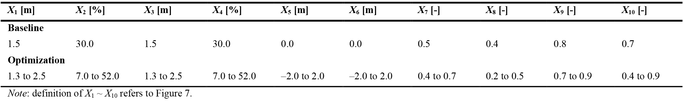
Table 4. The existing surface reflectance and transmittance values in typical classrooms in SDN 8.

Notice that the wall slopes (X₅ and X₆) are not measured in degrees. Instead, they are measured in terms of the distance (m) relative to the vertical walls (A and B, cf. Fig. 7) at the window elevation (X₁ and X₃). If the slope moves outside from the room, the slope is considered positive, and vice versa, as illustrated in Fig. 8.

Figure 8

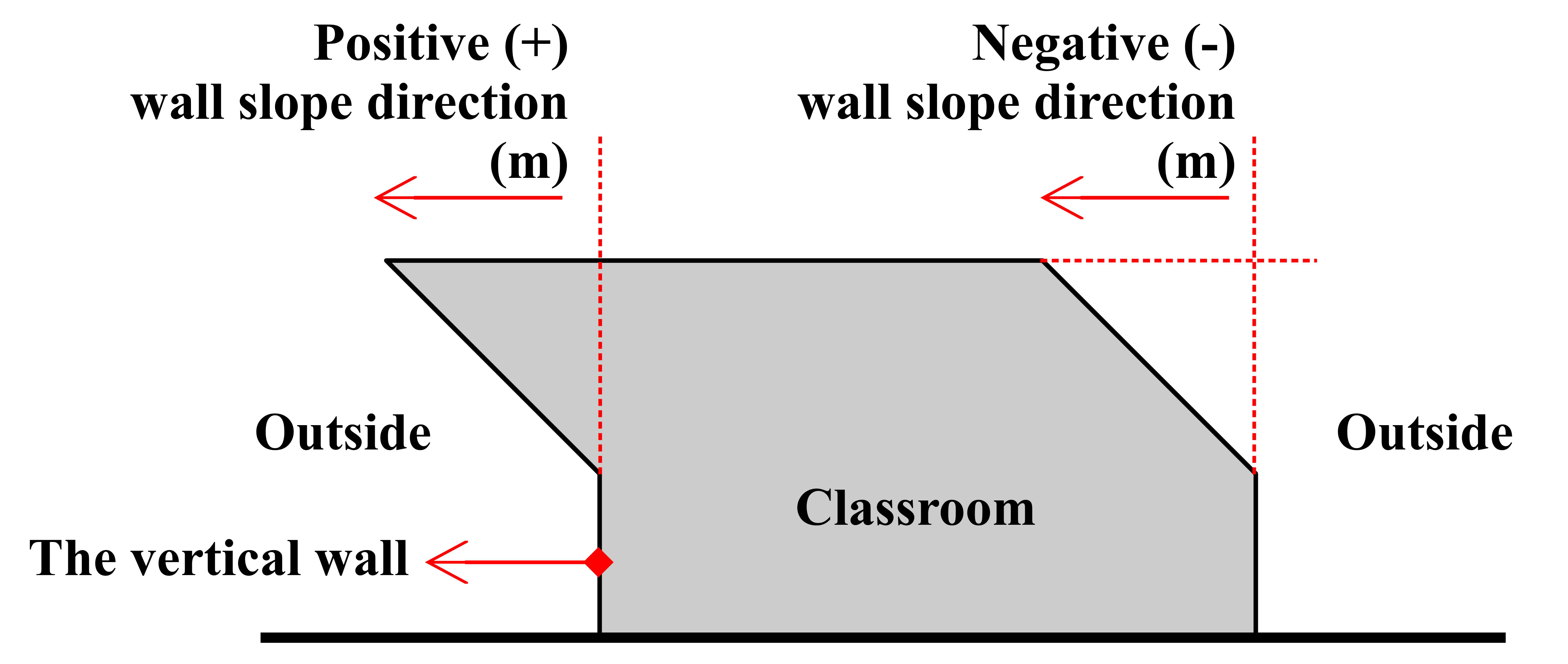
Fig. 8. Illustration of wall slopes.

To achieve the objective, computational modelling and simulation is employed. The simulation tool Honeybee [+] (HB[+]), with Radiance [59,60] as its engine, is employed to perform annual daylight calculation.

2.3. Simulation settings

For the annual daylight simulation, Radiance implements the rcontrib program that applies Monte Carlo raytracing algorithms, which applies random probabilistic sampling to solve the simulation problem [61]. Furthermore, the HB [+] employs the modified two phased dynamic daylight simulation (2PH-DDS-Mod) matrix method [59,62]. HB [+] assumes the presence of the real sun’s position throughout the year, also known as the analemma, instead of numerical approximation [59,63]. The sun’s position in the analemma is independent from the sky discretization [62], which has been verified for illuminance calculation [44].

Therefore, in this study, the default 145 sky patches are applied for the sky dome with the point-sun representation and its location in the analemma. The use of the 2PH-DDS-Mod matrix method, which is available within HB[+] interface, is considered appropriate since the geometrical model does not involve any complex fenestration system (CFS).

In this study, the weather data for Bandung and Lhokseumawe are utilized for the annual simulation. The data are extracted from the EnergyPlus weather (.epw) data of the relevant location. Next, during the utilization of daylight coefficient recipe in HB[+], the required Radiance ambient parameters are defined separately for three scenes: (i) normal scene, where all reflection is assigned as it is and the ambient bounce (ab) parameter is assigned as 6; (ii) black scenes, where all reflections are set to zero (ab = 1); and (iii) black analemma, where original sun positions across the sky dome is replaced with the sun on the analemma (ab = 0).

2.4. Optimization

The observed daylight metrics in this study are useful daylight illuminance (UDI), spatial daylight autonomy (sDA_300/50%), and annual sunlight exposure (ASE_1000,250). The classroom is assumed to be occupied from 8:00 to 17:00 hrs for the entire year, giving a total of 3650 hours. The UDI is defined as fraction of time in a year where the workplane illuminance at a given sensor point falls into certain illuminance ranges, due to daylighting only. A lower and an upper limit of the workplane illuminance is typically assumed for the computation [64,65]. In this study, the lower and upper limits are set to be 250 and 750 lux, as recommended by the Indonesian national criteria for daylighting in educational spaces [66]. Therefore, the UDI values in this case can be computed as per Eqs. (4)-(6):

\[ {\rm UDI}_{<250lx}=\frac{t_{E<250lx}}{T}\times100\%, \]

\[ {\rm UDI}_{250-750lx}=\frac{t_{250lx\le E<750lx}}{T}\times100\%, \]

\[ {\rm UDI}_{>750lx}=\frac{t_{E\geq750lx}}{T}\times100\%, \]

where t is duration in which the workplane daylight illuminance values satisfy the designated range, and T is the total duration in the year. Results from the UDI_250-750lx calculation are spatially averaged to yield , which is utilized for the optimization purpose.

Meanwhile, the sDA_300/50% and ASE_1000,250 criteria are set according to the LEED v4 [67]. The sDA_300/50% is a spatial-based DA metric, which itself is defined as percentage of time in a year satisfying the illuminance target of 300 lx or higher, using daylight only [68]. The DA₃₀₀ can thus be expressed in Eq. (7):

\[ {\rm DA}_{300}=\frac{t_{E>300\ lx}}{T}\times100\%, \]

where is the duration in which the workplane daylight illuminance values exceed 300 lux, and T is the total duration in the year. In addition, according to the Illuminating Engineering Society (IES), the DA₃₀₀ must fulfil at least 50% of the time annually, hence sDA_300/50%, as expressed in Eq. (8):

\[ sDA_{300/50\%}=\frac{A_{DA300\geq50\%}}{A_{total}} \times100\%, \]

where A_DA300≥50% is the sensor with DA₃₀₀ ≥ 50%, A_total is the total sensors inside the space. According to the IES, a minimum value of 55% is recommended for sDA_300/50%, in order to gain credits for daylighting [67].

Lastly, the ASE_1000,250 is described as the percentage of direct sunlight exposure at the workplane, with the threshold of 1000 lux for 250 hours per annum, without considering the interior and exterior reflections, i.e. the observed space is assumed to be a black room [67]. This metric serves as a criterion to observe for the potential of glare and overheat due to the excessive daylight [67,69]. The ASE_1000,250 thus reads as follows:

\[ {\rm ASE}_{1000,250}=\frac{A_{SE_{1000lx\geq250h}}}{A_{total}}\times100\%, \]

where A_{SE1000lx≥250h} is the sensor with direct sunlight illuminance value of 1000 lux for at least 250 hours in a year, and n_total is the total number of sensors in the workplane. Initially, the maximum criterion of ASE_1000,250 was set as 10%; however, since 2017, the criterion is revised so that the range between 10% to 20% is considered acceptable [69]. However, prior to calculating the metric, it is necessary to have daylight mitigation in the observed space by providing shading devices [69]. Since this study aims at the best-practice design solution without additional shading, therefore, 10% threshold is utilized. The internal shading devices, such as blinds, is not commonly used as a design practice, nor it is required by regulation in Indonesia (see Fig. 1) [39].

Furthermore, the values of and sDA_300/50% are maximized, while the ASE_1000,250 is minimized to obtain the optimum solutions. For the optimization purpose, an objective function Y is defined as follows:

\[ Y=\left(\overline{UDI}_{250-750lx}+sDA_{300/50\%}\right)-ASE_{1000,250} \]

To perform the multi-objectives optimization, the program Octopus for genetic algorithm (GA) is employed with strength Pareto evolutionary algorithm 2 (SPEA-2) algorithms. Octopus is selected since it is designed for multi-objective optimization with various embedded algorithms, such as SPEA-2. Also, Octopus has been widely utilized for building design optimization across the globe [2,11,18,70]. Thus, this study considers the utilization of Octopus for multi-objective optimization in this study is legitimate.

In each generation, 20 populations are set. After 15 generations, 15 out of 20 optimum solutions are selected for each building orientation, based on the resulting objective function Y. These optimum solutions are further analyzed to determine the sensitivity with respect to all considered input variables. The GA settings used for optimization in this study are shown in Table 5. The GA setting is as recommended by previous research on daylighting design optimization [71]. The optimizations are performed separately for each orientation in both cities.

Table 5

Table 5. GA settings for optimization in Octopus [71].

2.5. Visual comfort

The baseline and all optimum solutions obtained from the previous step are evaluated in terms of visual comfort condition on critical dates throughout the year: equinox on 21 March and two solstices on 22 June and December. In addition, since the sun altitude is relatively high in tropical regions such as Indonesia, the potential for glare inside space is most likely to happen in the morning and late afternoon. Thus, this study evaluates glare at those critical times at 9:00 and 15:00 hrs local time during the day. In addition, the baseline condition for all orientations in both cities are evaluated to compare with the optimum solutions in terms of the relevant glare metric.

The daylight glare probability (DGP) is employed as the glare metric, because it is purposefully proposed for daylight glare evaluation inside a space [72].

\[ DGP=5.87\times10^{–5} E_v+ 9.8 ×10^{–2} log\left(\mathrm{1\ +\ }\sum_{\mathrm{i}}\frac{\mathrm{L}_{\mathrm{s,i\ }}^\mathrm{2}\mathrm{\omega}_{\mathrm{s,i}}}{{\mathrm{E}_\mathrm{v}^{\mathrm{1.87}}\mathrm{P}\ }_\mathrm{i}^\mathrm{2}}\right)+0.16, \]

where E_v is the vertical illuminance on the observer’s eye, L_s,i is the source luminance, is the solid angle, and P_i is the Guth position index. The calculation point for DGP evaluation is located in the center of the classroom, elevated at 1.2 m (Fig. 9). The arrow (blue) shows the view direction of the camera. For orientations other than 0°, the view direction follows counterclockwise rotation. Furthermore, the DGP is calculated using rpict function of Radiance utilizing the high setting shown in Table 2, based on the verification result. The rpict script is utilized to generate high dynamic range (HDR) images for DGP calculation in the later stage using Evalglare., which is accessed through HB Glare Postprocess component of Ladybug Tools. Finally, the false color images are generated using falsecolor script of Radiance through the Ladybug Tools component.

Figure 9

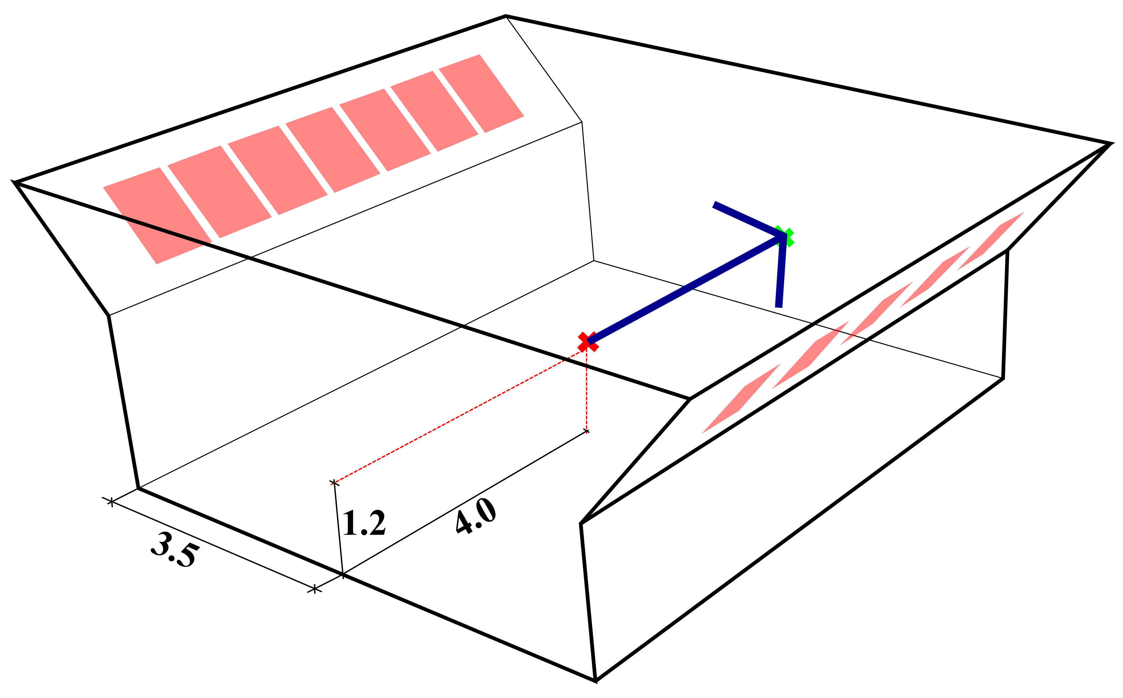
Fig. 9. Perspective view of the DGP calculation point and its view direction.

The DGP in this study acts as an indicator of visual discomfort, though it is not directly included in the optimization process. The main reason for not including DGP in the definition of Y value is due to the high computation cost for predicting the annual performance. Instead, the verification is only conducted for the critical dates as mentioned earlier.

For the DGP category, this study adopts the range of criteria previously proposed for the tropical condition in Bandung [73]. The referred study is considered as a pilot study in Indonesia, which investigated daylight discomfort glare and proposed the relevant categories for the local context, which is rather different from the original DGP criteria [72]. The implemented categories are tabulated in Table 6.

Table 6

Table 6. GA settings for optimization in Octopus [71].

2.6. Data analysis

For the data analysis, this study employs multiple stages analysis, namely correlation, sensitivity, and uncertainty analysis. The multiple stages analysis is conducted due to the input variables’ tendency to have non-parametric relations with the output. Thus, the correlation is meant to filter for potential parametric input variables that can be utilized later for sensitivity analysis. The variables in the sensitivity analysis are considered to have parametric relation with the output parameters. The uncertainty analysis is utilized to observe the sensitivity of output variables with respect to the input.

First, the Spearman rank correlation coefficient (r_s) is applied to analyse the correlation at each building orientation in both cities. The correlation is observed for the objective function Y, which has been defined in Equation (9). Next, four levels of assessment scale (Table 7) are employed to interpret the correlation strength as indicated by the absolute r_s values from the observed data. Values of |r_s| ≥ 0.70 indicates a strong correlation between the input and output variables, whereas |r_s| ≤ 0.29 indicates a very weak correlation. The correlation analysis is employed as a filter for the strong and moderate correlated of input and output parameters to be taken for further sensitivity analysis.

Table 7

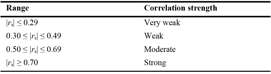
Table 7. Assessment scale for interpretation of the Spearman rank correlation coefficient (r_s).

Next, for sensitivity analysis, this study utilizes multi-linear regression model. If more than one input is available, the variables with strong and moderate correlations are evaluated according to Eq. (12). Otherwise, a simple linear regression model is applied. The multi-linear regression model reads:

\[ Y_i=\beta_1X_{1i}+\beta_2X_{2i}+\beta_3X_{3i}+\ldots+\beta_qX_{qi}+\varepsilon_i\ ,\ i=1,2,3,\ldots,n. \]

where ε_i is the residual error or intercept, q is the number of input variables, and n is the number of variations within each input variable.

Since the variables have diverse units, it is required to standardize the input and output variables. The coefficients are called standardized regression coefficient (SRC), ranging from –1 to +1. The closest the SRC to –1 or +1, the more sensitive the output variable to the change of the input variable. As explained, the i-th input and output variables are denoted respectively as x_i and y_i. The standardization is defined in Eq. (13) for the input variables and in Equation (14) for the output variables.

\[ X_{ji}^\prime=\frac{X_{ji}-\bar{X}j}{{\sigma_X}_j},\ i=1,2,3,\ldots,\ n;\ j=1,2,3,\ldots,q \]

where X'_ji is the standardized j-th input variable of the i-th variation, X_ji is the original j-th input variable of the i-th variation, is the mean of the j-th input variable, and σ_Xj is the standard deviation of the j-th input variable.

\[ Y_i^\prime=\frac{Y_i-\bar{Y}}{\sigma_Y}\ ,\ i=1,2,3,\ldots,\ n \]

where Y_i' is the standardized output variable, Y_i is the i-th original output variable, Ῡ is the mean value of the output variable, and σ_Y is the standard deviation of the output variable. The standardization principle also applies for the simple linear regression, in which only a single input variable is involved.

Finally, uncertainty analysis is evaluated for 15 optimum solutions at each orientation in each city by observing the coefficient of variance (CV) and visualization of optimum solutions using points plot. The CV is defined as the ratio between the standard deviation and the mean values of the data. In this case, the intended output is the Y values at every orientation in both cities. Furthermore, the top five optimum solutions are also observed to understand input and output parameter configuration at each orientation in both cities. To obtain a comparable input and output parameter, thus, the original domain of input and output variables are transferred into a normalized range between 0 and 1. In order to achieve this, Eq. (15) is utilized:

\[ N=\left(\frac{C-X_{min}}{X_{max}-X_{min}}\right).\ \left(Y_{max}-Y_{min}\right)+\ Y_{min} \]

where N is the normalized value, C is the original number input to be normalized. X_min and X_max are the original minimum and maximum thresholds, while Y_min and Y_maxare the normalized, target minimum and maximum thresholds.

3. Results

3.1. Verification and validation

3.1.1. Verification

Comparison between analytical and simulated SC values for all settings (low, medium, and high) is depicted in Fig. 10(a). It is shown that simulation results generally follow the similar trend of the analytical ones. The farther the distance of the sensors from the daylight opening, the lesser the SC values, except at sensor A that is the closest to the façade. Although it has similar trend between analytical calculation and the simulation result at sensor A (the nearest to the opening), the SC value has the greatest error around 54~56% (see Fig. 10(b)), which is unacceptable. It is observed that the distance from the opening to sensor A is 0.25 m, while an earlier study has suggested that perimeter sensors should be located at least 0.50 m from the façade wall [74]. Therefore, the perimeter sensors particularly the one next to the opening must be equal or above 0.50 m. Thus, this study adopts this rule to avoid discrepancy in the simulation.Aligning with the current studies that necessitate daylight performance analysis combined with visual comfort, the present

Figure 10

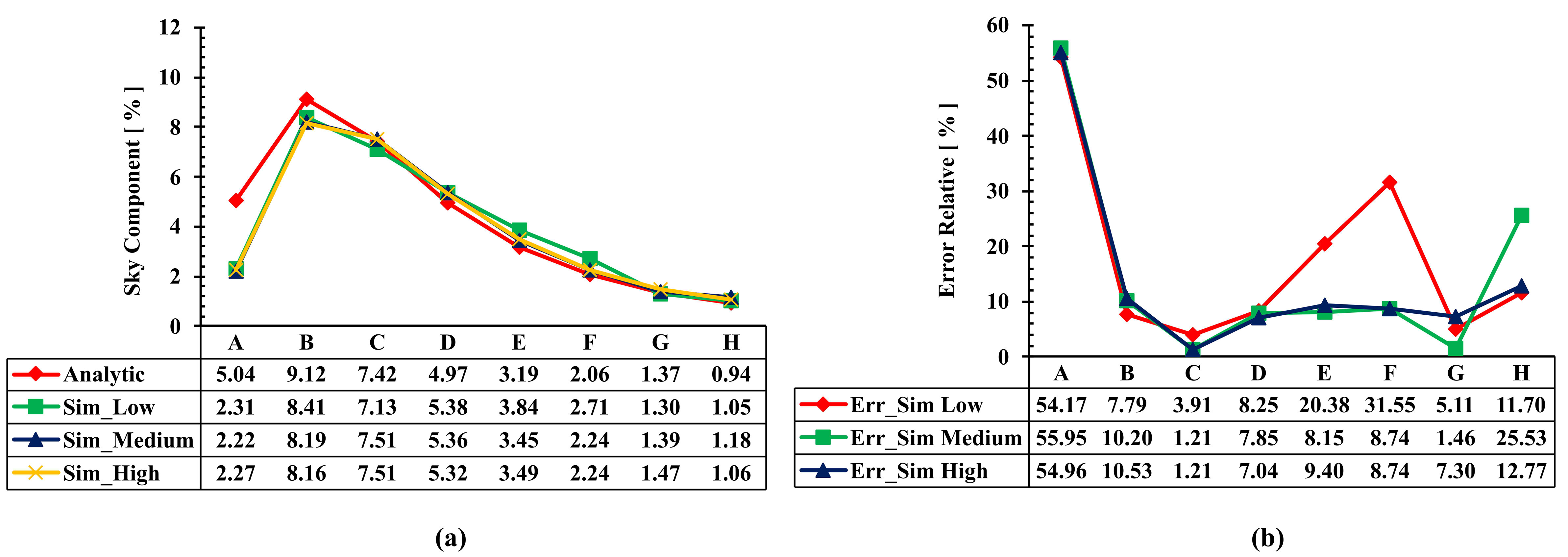
Fig. 10. (a) Analytical and simulated SC values and (b) the relative errors at all sensor points inside the hypothetical room of the CIE test case 5.13.

Next, except for sensor A, it is discovered that the high Radiance setting indicates the least fluctuating SC values within the hypothetical room, which are under 15% on average. This is significant to consider in the simulation, since it may lead to inaccurate overall results, if the inconsistency appears throughout the sensors. Thus, for accurate and consistent simulation results, this work employs high simulation setting of HB [+]. Comparison of errors between low, medium, and high Radiance settings is displayed in Fig. 10(b).

3.1.2. Validation

For modelling the field measurement in SDN 8, the high simulation setting is utilized based on previous analytical verification result. Figures 11(a) and (b) show that the average DF value at each sensor point has different trend, except at sensor F between the field measurement and simulation. However, when analyzed for the average DF values, the errors are found only less than 1.50%, as shown in Fig. 11(c).

Figure 11

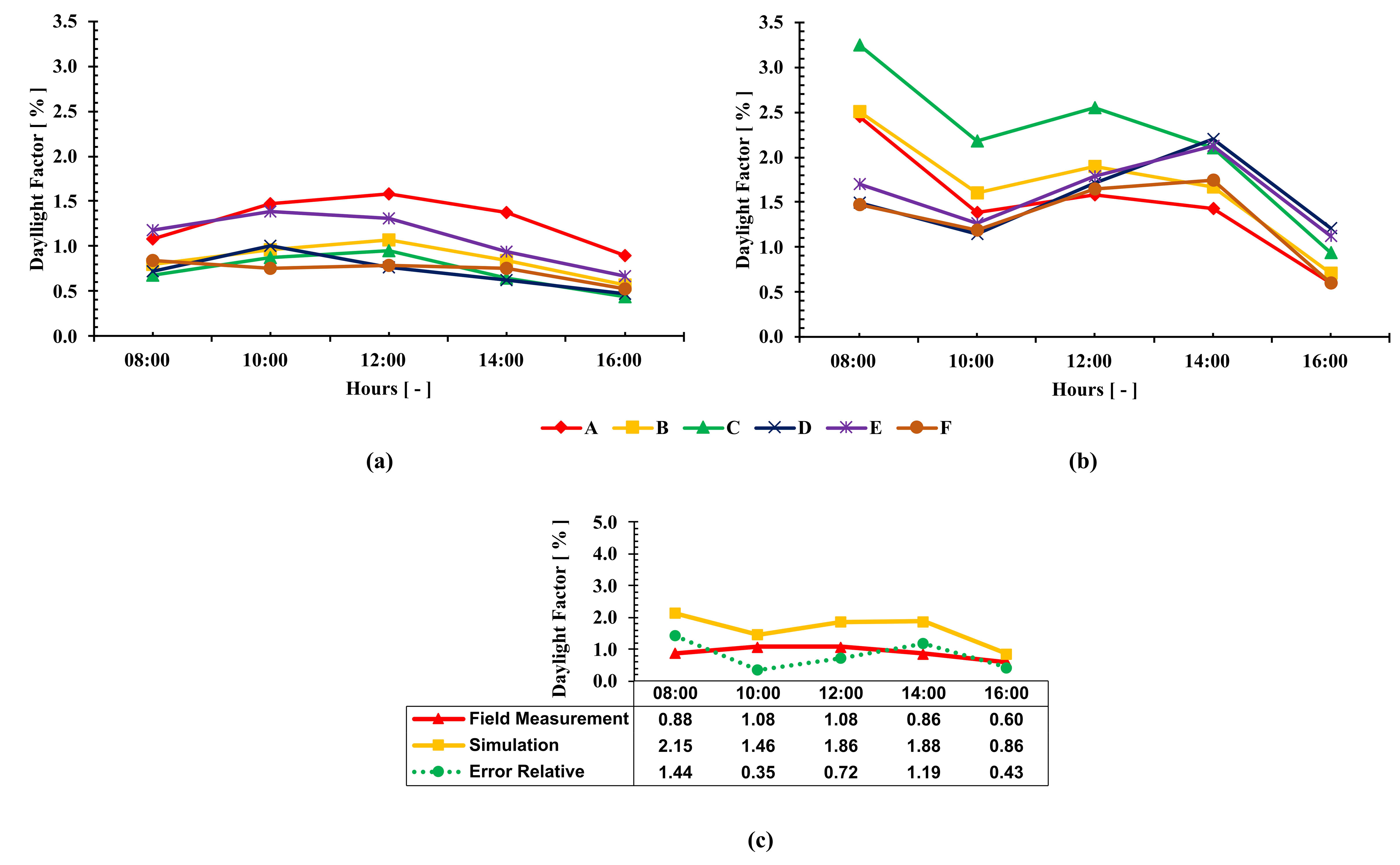
Hourly average DF at each sensor point (A-F) based on (a) field measurement and (b) simulation, and (c) average DF from field measurement and simulation, and the resulting error at each observed hour in SDN 8.

Fig. 11. Hourly average DF at each sensor point (A-F) based on (a) field measurement and (b) simulation, and (c) average DF from field measurement and simulation, and the resulting error at each observed hour in SDN 8.

Based on the analytical verification and experimental validation, the Radiance simulation setting is verified and validated for the purpose of this study. Therefore, the Radiance engine can be applied for annual daylight simulation through the interface of HB [+]. Moreover, Radiance has been utilized by many scholars for daylighting analysis in various scenarios and regions of the world [9,14,35,62,74–76], and has also been embedded in various end-user daylight simulation tools. For the accuracy and consistency of simulation result, the high Radiance setting is employed as suggested from the verification results.

3.2. Baseline

3.2.1. Daylight metrics

For the baseline result, small values of the objective function Y are found at all orientations in both cities. Table 8 shows low and high (< 5%) and sDA_300/50%(100%), respectively, meaning that in the baseline scenario, excessive daylight occurs at the modelled classroom in both cities. Furthermore, the Y value in Lhokseumawe is lower compared to that in Bandung. This is because in Lhokseumawe, the average ASE_1000,250 values at all orientations are higher. At orientation 90º, both cities have greater Y values, since the window locations are orientated away from the east and west. Conversely, results at orientation 0º suggest the opposite trend from those at orientation 90º.

Table 8

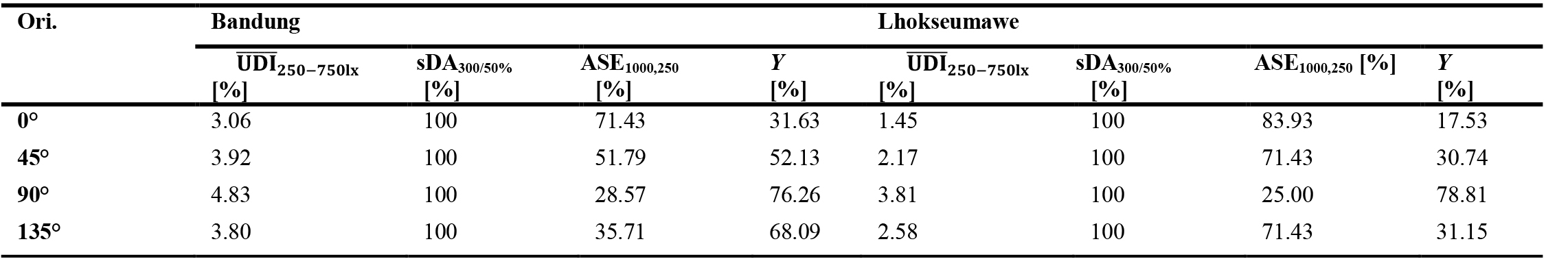
Table 8. Baseline results of the annual daylight metrics and objective Y at all orientations in Bandung and Lhokseumawe.

3.2.2. Daylight glare probability

In the baseline scenario in Bandung, DGP values that fall into disturbing category is found at almost all investigated times of the year, at all orientations (Figs. 12(a) and (b)). The lowest DGP is discovered on 22 June at 15:00 hrs (DGP = 0.22) at orientation 45º. On the other hand, the most disturbing glare occurs on the same day at 09:00 hrs (DGP = 0.32) also at orientation 45º. The falsecolor image of the most disturbing glare scene in Bandung is shown in Fig. 12(c), referring to the view direction in Fig. 9.

Figure 12

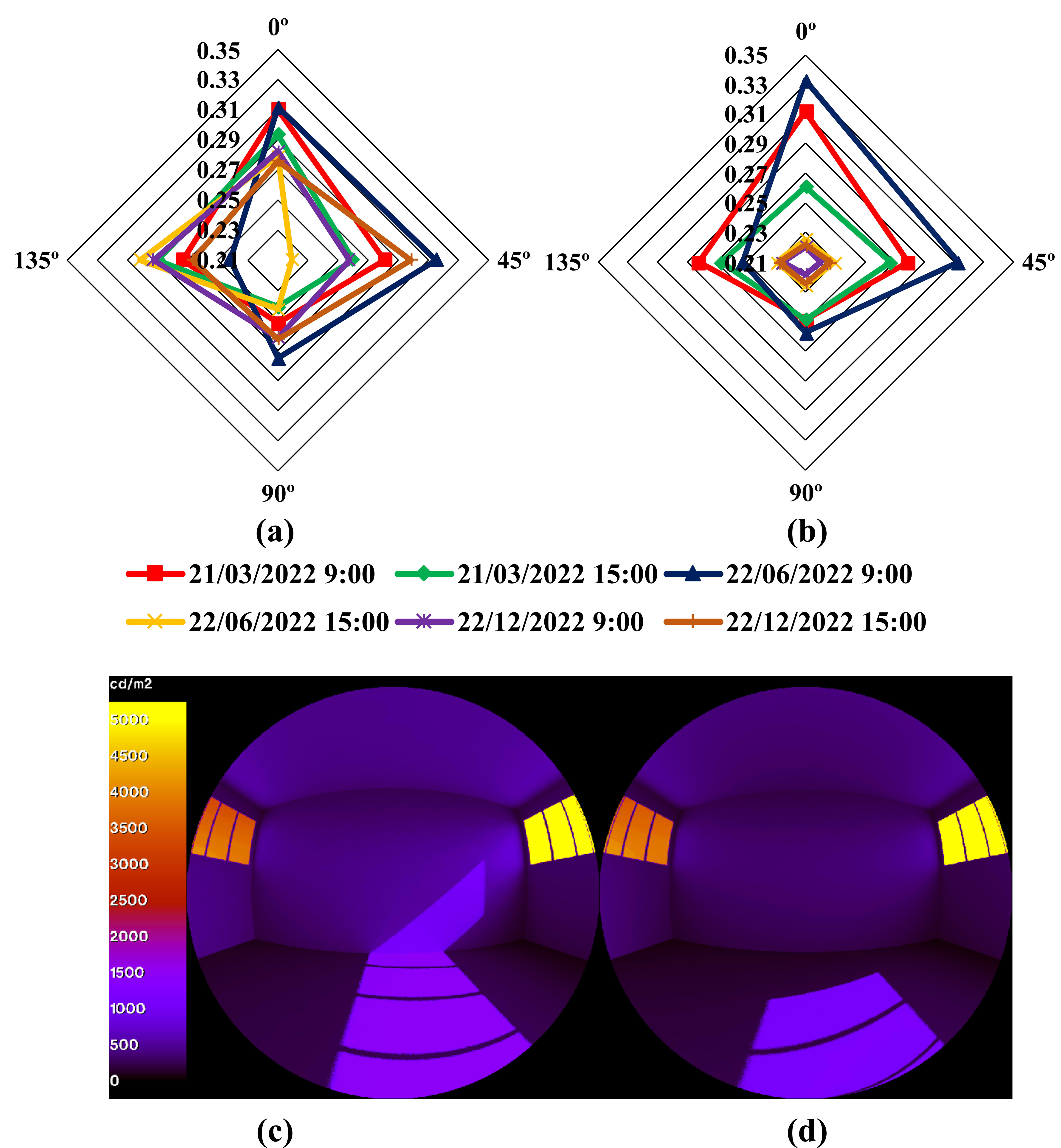
Baseline DGP values in (a) Bandung and (b) Lhokseumawe, and the falsecolor image with the highest DGP values in Bandung ((c); DGP = 0.32) and Lhokseumawe ((d); DGP = 0.33) at orientation 45º and 0º respectively, both occurs on 21 June at 09:00 hrs.

Fig. 12. Baseline DGP values in (a) Bandung and (b) Lhokseumawe, and the falsecolor image with the highest DGP values in Bandung ((c); DGP = 0.32) and Lhokseumawe ((d); DGP = 0.33) at orientation 45º and 0º respectively, both occurs on 21 June at 09:00 hrs.

Meanwhile, for the baseline in Lhokseumawe, the low DGP values occur on 22 June at 15:00 hrs, and on 22 December at 09:00 and 15:00 hrs at all orientations (DGP = 0.22 ~ 0.23; Fig. 12(c)). Meanwhile, the highest DGP is found at orientation 0º on 22 June at 09:00 hrs (DGP = 0.33). Also, during equinox in Lhokseumawe, relatively high glare occurs in the morning (DGP = 0.31). Similarly, on 22 June at 09:00 hrs, the DGP is relatively high in Lhokseumawe. False color image visualization of the most disturbing glare scene in Lhokseumawe is depicted in Fig. 12(d), also referring to Fig. 9 for view direction.

In Bandung, most of DGP values fall under the disturbing-intolerable category, except on 22 June afternoon, in which the DGP value falls under the imperceptible-perceptible category (DGP = 0.22). Meanwhile, in Lhokseumawe, the DGP values on 21 March at 09:00 and 15:00 hrs and on 22 June at 09:00 hrs are under the disturbing-intolerable category. The rest falls under the imperceptible-perceptible category.

3.3. Optimum solutions

3.3.1. Daylight metrics

Based on the optimization result for both cities, the minimum, mean, and maximum objective function (Y) values, in %, are tabulated in Table 9. Meanwhile, the corresponding input variables for the maximum Y values are reported in Table 10.

Table 9

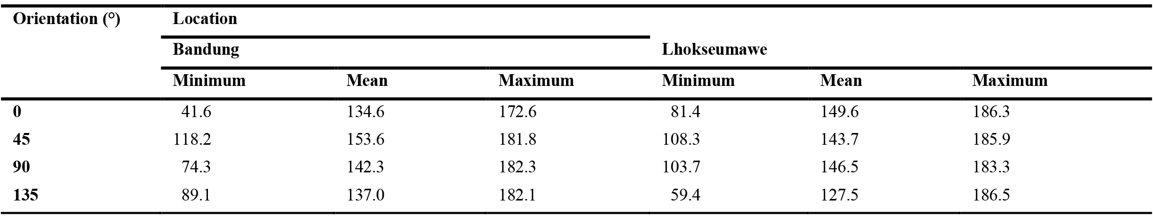
Table 9. Minimum, mean and maximum Y values (%) at each orientation in Bandung and Lhokseumawe.

Table 10

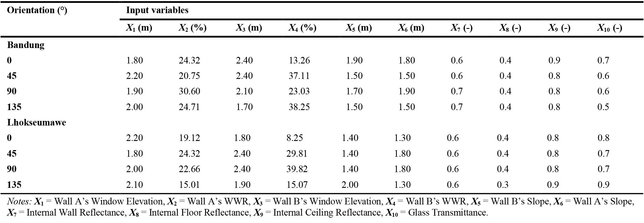
Table 10. Input variables corresponding with the maximum Y values in Bandung and Lhokseumawe.

3.3.2. Daylight glare probability

The DGP values in the optimum solutions in Bandung and Lhokseumawe at all orientations are shown in Figs. 13(a) and (b). It is observed from Fig. 13(a) that in the optimum solutions in both cities, all DGP values have been improved (DGP < 0.24) into the category of imperceptible and imperceptible-perceptible at some evaluated hours. In Bandung, the previously most disturbing glare condition, at orientation 45º, has been improved from DGP = 0.32 to 0.20, which occurs on 22 June at 09:00 hrs. Similarly, in Lhokseumawe, the DGP has been improved from 0.33 to 0.22, which occurs at orientation 0º on 22 June in the morning.

Figure 13

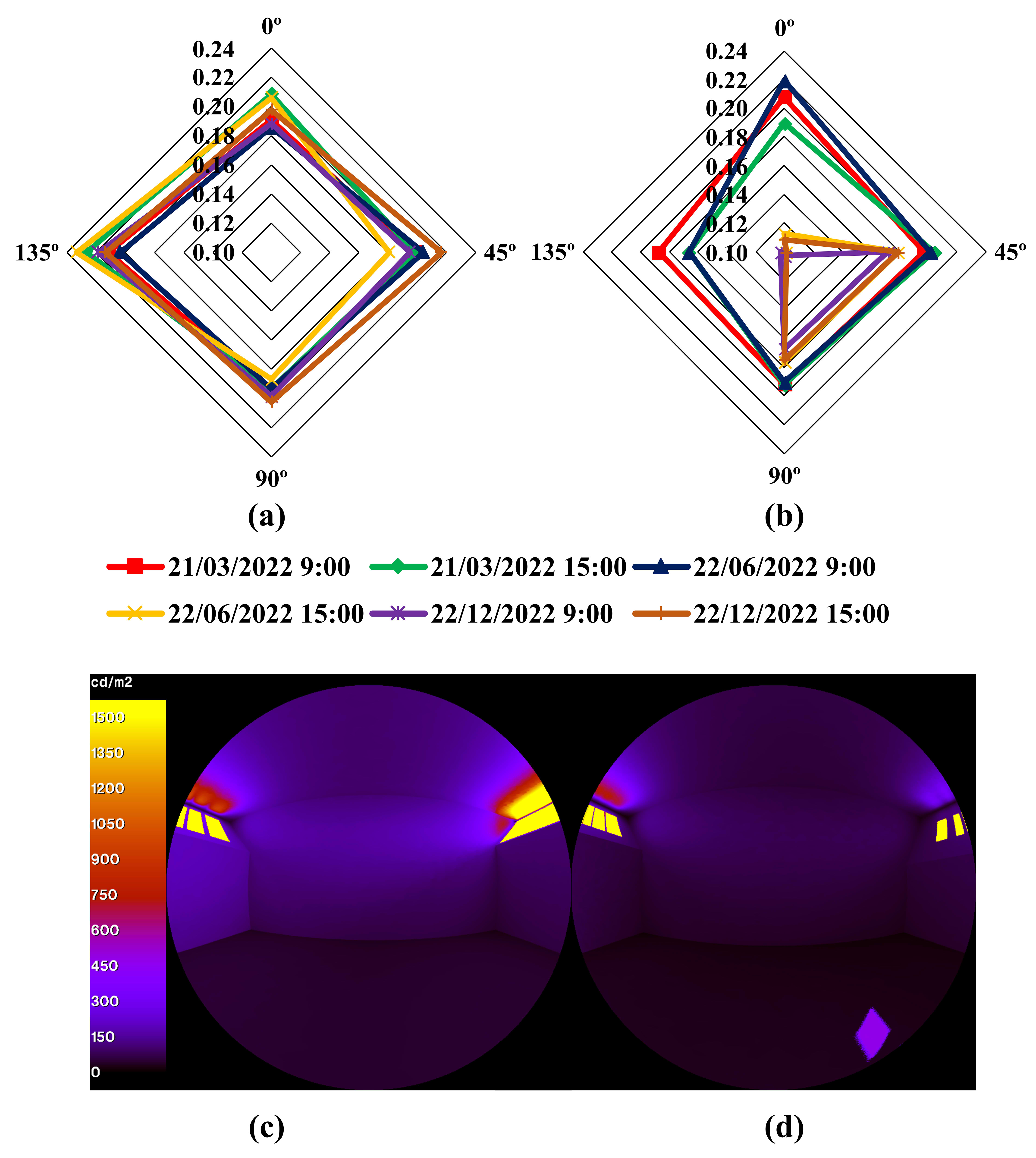
DGP values for the optimum solutions in Bandung (a) and Lhokseumawe (b) at all orientations, and the falsecolor images of the most disturbing glare in Bandung ((c) DGP = 0.20) and Lhokseumawe ((d) DGP = 0.22) at orientation 45º and 0º respectively, on 21 June at 09:00 hrs.

Fig. 13. DGP values for the optimum solutions in Bandung (a) and Lhokseumawe (b) at all orientations, and the falsecolor images of the most disturbing glare in Bandung ((c) DGP = 0.20) and Lhokseumawe ((d) DGP = 0.22) at orientation 45º and 0º respectively, on 21 June at 09:00 hrs.

Furthermore, Fig. 13(b) displays that the improvement is slightly better in Lhokseumawe than that in Bandung, in terms of DGP values at the evaluated critical hours of the year. There is no DGP values equal or above 0.23 in Lhokseumawe at any time. Meanwhile, the highest DGP value in Bandung is 0.23, which happens in the afternoon on 21 March and 22 June at orientation 135º (Fig. 13(a)). To provide a better perspective, the false color image of the DGP in the optimum solutions in both cities is depicted in Figs. 13(c) and (d).

It is also observed that the DGP values in Lhokseumawe at all orientations are lower than those in Bandung. This is mainly because both cities use the same local time, which is UTC+7, but Bandung is located at longitude 107.6°E, which is near its reference meridian (105°E); whereas Lhokseumawe is located at longitude 97.1°E. Thus, at same time of the day in the morning, illuminance values in Bandung are relatively higher than those in Lhokseumawe, because the solar time in Lhokseumawe is well behind its clock time. Moreover, Bandung is also located at a higher elevation (675~1050 m above sea level) than Lhokseumawe (2~24 m above sea level), so that the former receives relatively greater solar radiation than the latter, as confirmed in Figs. 6(a) and (c).

3.4. Analysis

It is found that at least two input variables have a strong or moderate correlation, except at orientation 135°, in which there is only one input variable with strong or moderate correlation in both cities. Meanwhile, at orientation 45°, there are no input variables with strong or moderate correlation in Lhokseumawe. Overall, the results suggest that each variable has a different level of correlation, while both cities also yield different profile of correlation. The obtained profiles of the Spearman rank correlation coefficient (r_s) for all input variables in both cities are shown in Fig. 14.

Figure 14

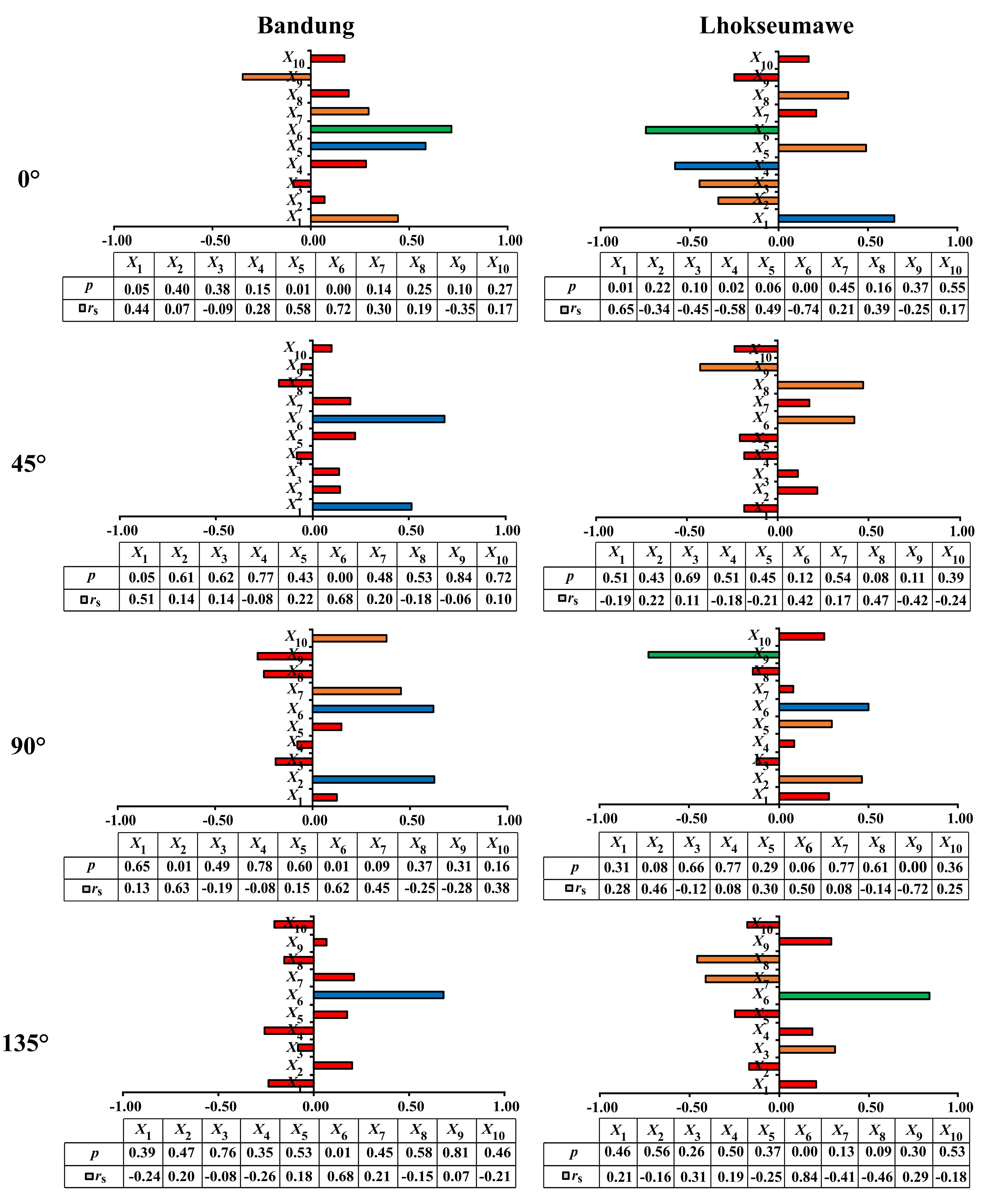
Fig. 14. Spearman rank correlation coefficient (r_s) for each building orientation in Bandung and Lhokseumawe.

At orientation 0°, the highest r_s value is found for the wall A’s slope (X₆), in Bandung (r_s = 0.72, p < 0.01) and Lhokseumawe (r_s= –0.74, p < 0.01). This indicates a strong correlation between the objective function Y and the wall A’s slope, in a positive trend for Bandung and in a negative trend for Lhokseumawe. At orientation 45°, no strong correlations are found for any variables in both cities; while at orientation 90°, strong correlation is only found for the ceiling reflectance (X₉, r_s = –0.72, p < 0.01), in Lhokseumawe. Finally, at orientation 135°, strong correlation is also only found in Lhokseumawe, for the wall A’s slope (r_s = 0.84, p < 0.01).

The moderate correlations (blue bars in Fig. 14) for each orientation in both cities are also different. At orientation 0°, the wall B’s slope (X₅, r_s = 0.58, p = 0.01) in Bandung and the wall A’s window elevation (X₁, r_s = 0.65, p = 0.01), as well as the wall B’s WWR (X₄, r_s = –0.58, p = 0.02) in Lhokseumawe are found to be the input variables with moderate correlation with the objective function. At orientation 45°, the wall A’s window elevation (r_s = 0.51, p = 0.05) and its slope (r_s = 0.68, p < 0.01) are the input variables with moderate correlation in Bandung. Meanwhile, at the same orientation, there are no input variables with moderate correlation in the location of Lhokseumawe.

At orientation 90° in Bandung, moderate correlation is found for two input variables, which are the wall A’s WWR (X₂, r_s = 0.63, p = 0.01) and its slope (X₆, r_s= 0.62, p = 0.01). Meanwhile, at the same orientation in Lhokseumawe, moderate correlation is only found for the wall A’s slope (r_s = 0.50, p = 0.06). However, as the p-value for that variable is more than 0.05, it is therefore considered statistically insignificant.

Lastly, at orientation 135° in Bandung, moderate correlation is only found for the wall A’s slope (r_s= 0.68, p = 0.01). Meanwhile, similar to the orientation 90°, there are no input variables with moderate correlation in Lhokseumawe. The rest of input variables fall under the categories of weak and very weak correlations (orange and red bars in Fig. 14), so that their contributions are considered insignificant.

Furthermore, from the sensitivity analysis, the highest coefficient of determination R²= 0.68 is found at orientation 0° in Bandung and 90° in Lhokseumawe, whereas the lowest R²= 0.53 is found at orientation 90° in Bandung. It means the multilinear models can moderately explain the phenomena being examined. The complete sensitivity analysis parameters (SRC, R², and p) is shown in Table 11 for both cities at all orientations.

Table 11

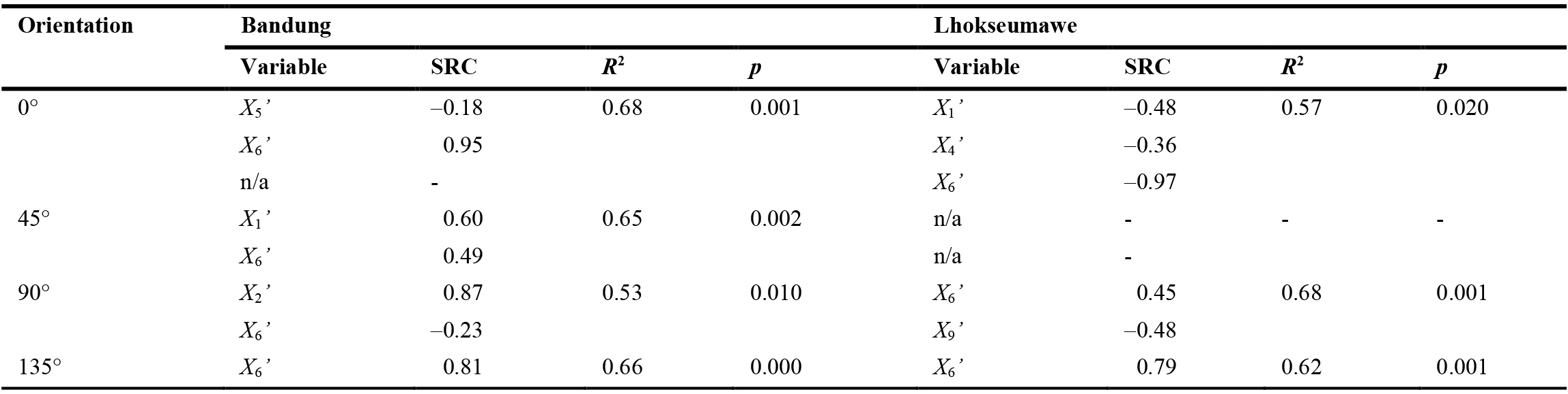
Table 11. Variables and SRC values for Bandung and Lhokseumawe at all orientations.

Table 11 suggests at orientation 0°, the wall A’s slope (X₆’) is the most sensitive variable for both cities. The impact on Y values is found to be highly positive (SRC = 0.95, R²= 0.68) in Bandung but highly negative (SRC = –0.97, R²= 0.57) in Lhokseumawe, which is somewhat similar with the Spearman correlation analysis. Obviously, the moderately correlated input variables yield less influence on the daylight metrics in both cities.

At orientation 45°, the wall A’s window elevation (X₁’) has a moderate influence on Y values in Bandung (SRC = 0.60, R²= 0.65); while there are no input variables having strong or moderate impact on Y values in Lhokseumawe. At orientation 90°, the wall A’s WWR (X₂’) has a strong impact (SRC = 0.87, R²= 0.53) on Y values in Bandung. However, at the same building orientation in Lhokseumawe, no input variables have a strong or moderate impact, even though the ceiling reflectance (X₉’) does have a high Spearman rank correlation. There is also inconsistency in trends between correlation and sensitivity analysis for the wall A’s slope (X₆’) in Bandung. However, the variable only shows a low sensitivity (SRC = –0.23).

Furthermore, at orientation 135°, it is found that the wall A’s slope has a strong impact on Y values in Bandung (SRC = 0.81, R²= 0.66) and Lhokseumawe (SRC = 0.62, R²= 0.62). At orientation 45°, as has been explained earlier, none of the input variables have a strong influence on the output in both cities. At orientation 90°, only Bandung has a strongly influential variable, which is the wall A’s WWR (X₂’).

Next, to understand the uncertainty, Fig. 15 illustrates all optimum solutions, sorted from the smallest to the greatest Y values, for both cities. It shows that all optimum solutions in all orientations tend to diverge from their optimum values. Particularly, in Bandung for design option 1, 2 and 3 in orientation 0°, and design option 1 and 2 for orientation 90°, which is dramatically inclined as illustrated in Fig. 15(a). Also, Figs. 15(a) and (b) shows that the optimum Y values from the 15 optimum solutions tend to diverge at all orientations in both cities. Therefore, CV values shall be computed to understand the uncertainty of the optimum conditions.

Figure 15

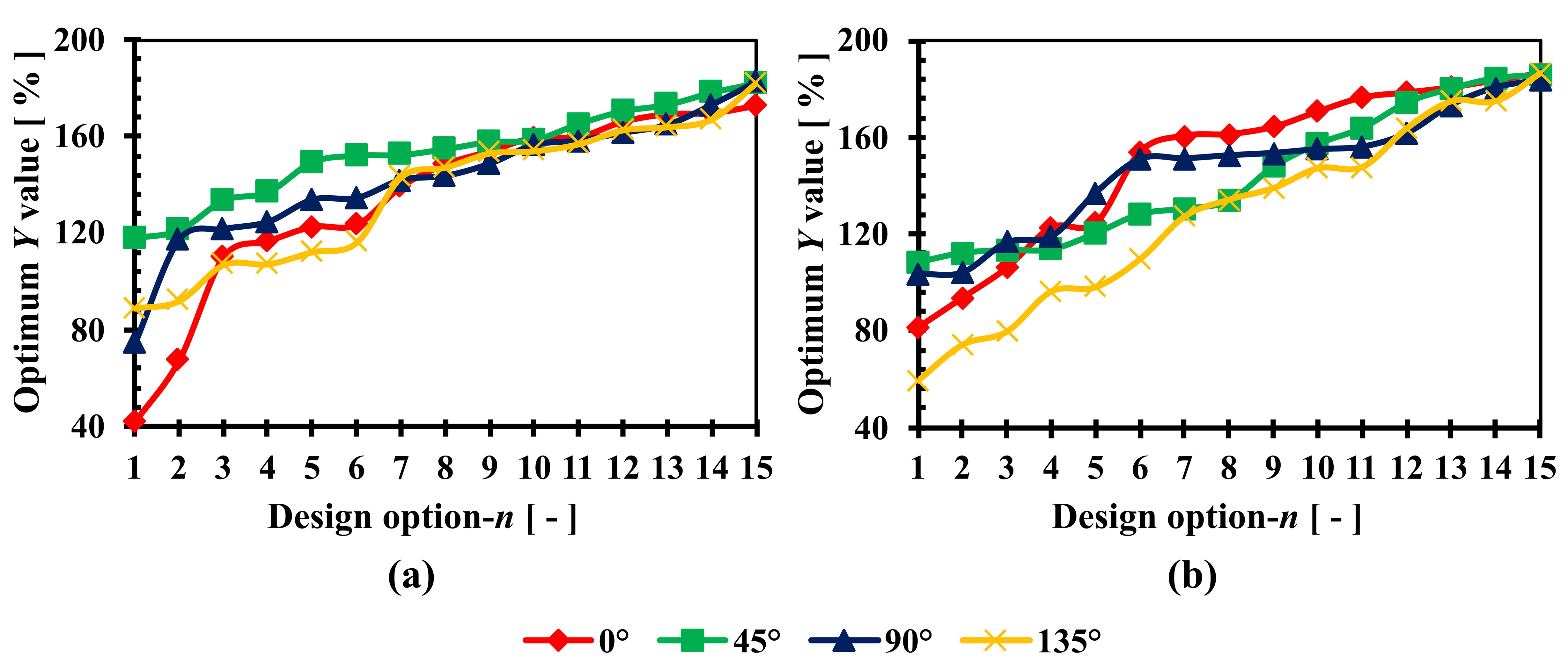
Fig. 15. All optimum solutions for Bandung (a) and Lhokseumawe (b) at all relevant orientations.

Table 12 shows that the CV values are relatively high for the 15 optimum solutions, at above 0.10, in both cities at all orientations. This means the strong influential input variables still can change the objective value significantly without a proper design attention is given. In Bandung, the highest uncertainty of objective Y value occurs at orientation 0º (CV = 0.29), which is indicated by the Y range in Fig. 15(a) (41~172%). On the other hand, in Lhokseumawe, the highest uncertainty (CV = 0.31) is discovered at orientation 135º (Y values within 59~186%) as illustrated in Fig. 15(b). Furthermore, CV values at orientation 45º and 135 º in Bandung are less than those in Lhokseumawe. Conversely, at orientation 0º and 90º, Lhokseumawe has a lower uncertainty compared to Bandung.

Table 12

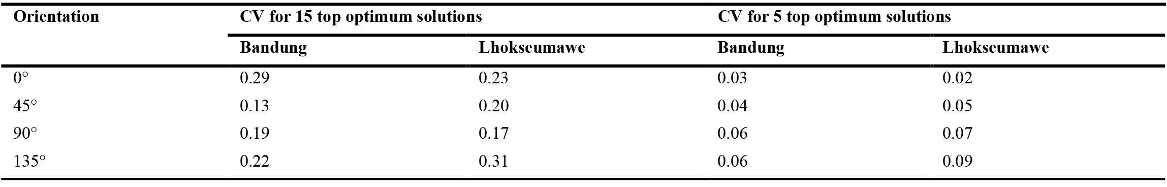
Table 12. CV values of the objective function Y at all orientations for the top 15 and 5 optimum solutions in Bandung and Lhokseumawe.

However, when further analysis is conducted from the top five optimum solutions in Bandung and Lhokseumawe, the CV value of objective Y has decreased significantly below 0.10 at all orientations (Table 12). For the top five optimum solutions, the CV values trend is similar to the 15 optimum solutions, except at orientation 90º, where the CV value in Bandung has been slightly lower than that in Lhokseumawe.

Next, Fig. 16 depicts the first optimum solutions (Option 15), the input parameter combinations at each orientation in both cities are all different. Therefore, to realize a daylight-friendly design in classrooms with bilateral opening, the combination of design parameters should be carefully considered at each façade orientation. In other words, the design solution for a certain façade orientation may not be generalized for other orientations.

Figure 16

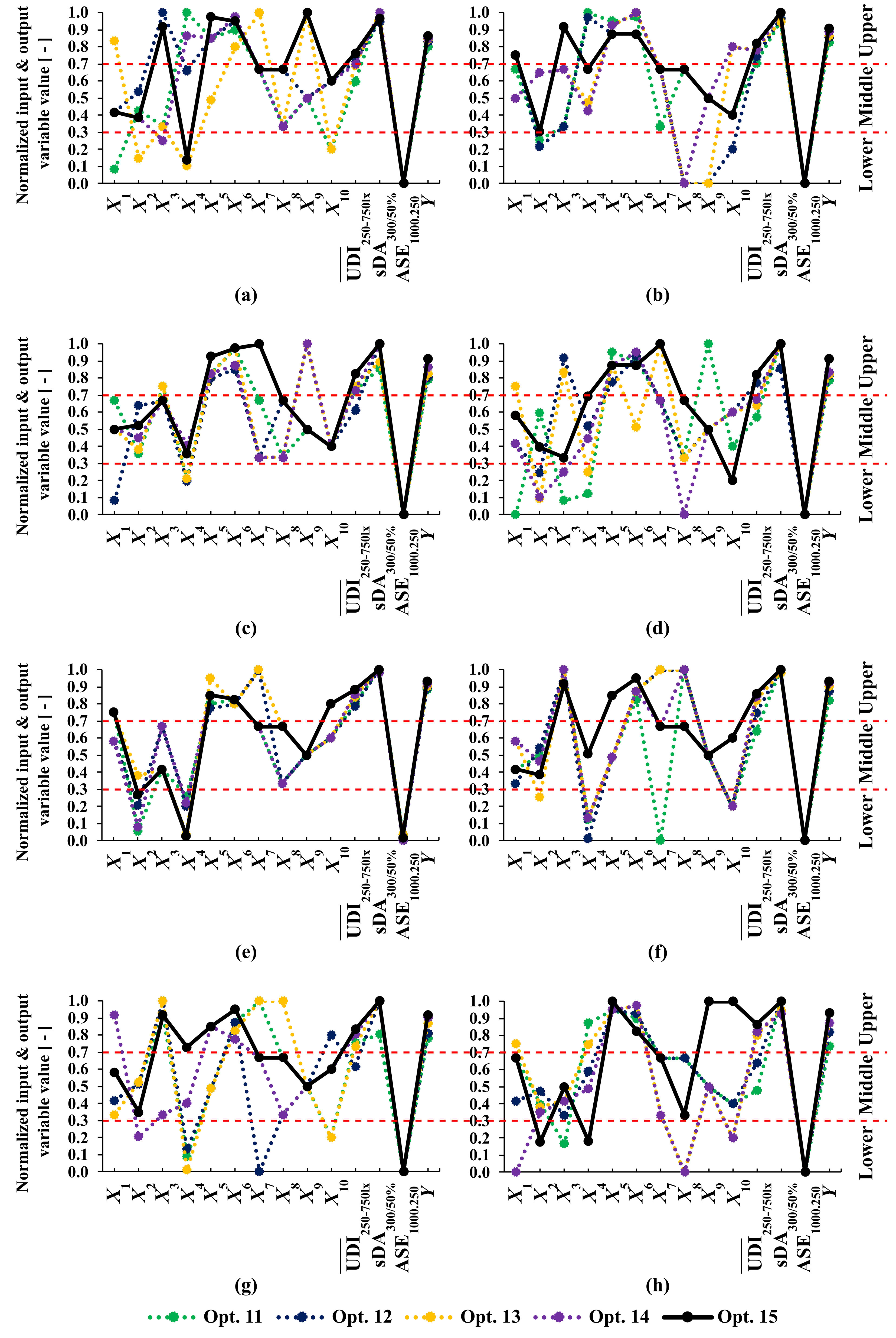
Top five optimum solutions in Bandung (design option 11 to 15) at orientation (a) 0º, (b) 45º, (c) 90º, and (d) 135º, and those in Lhokseumawe at orientation (e) 0º, (f) 45º, (g) 90º, and (h) 135º.

Fig. 16. Top five optimum solutions in Bandung (design option 11 to 15) at orientation (a) 0º, (b) 45º, (c) 90º, and (d) 135º, and those in Lhokseumawe at orientation (e) 0º, (f) 45º, (g) 90º, and (h) 135º.

From the top five optimum solution (Option 11 until 15), the most uncertain metric is . Thus, attention should be paid on that metric because a slight change in the input variables may significantly alter the outcome (CV > 0.1). This is particularly true as far as the most influential input variables, such as the wall slope and WWR, are involved. This finding also applies to both cities, except at orientation 45º in Bandung (Fig. 16(b)) and at orientation 0º in Lhokseumawe (Fig. 16(e)), where the tend to deviate less. However, if only objective Y is observed, the predicted optimum solutions tend to converge with less uncertainty (CV < 0.1).

Also, from the top optimum solutions, it is found that most of the optimum input variables are in the middle and upper value categories, at all orientations in both cities. Meanwhile, in terms of WWR, different optimum window configurations can be suggested for wall A and B in both cities. Thus, a non-symmetrical facade design solution is recommended.

A higher transmittance value (Option 15) is preferable for the window glass material in both cities since the glass transmittance values are in the upper and middle categories. An exception is found at orientation 135º in Bandung, where a low transmittance value is recommended to achieve the optimum solution. This solution shall balance the large WWR of wall B on the northwest façade, where a great amount of direct sunlight may occur in that direction in the middle of the year, since Bandung is located at the south of the equator.

4. Discussion

As described in the Introduction, this study focuses on optimizing daylighting performance in school classrooms with bilateral opening, which are rarely investigated in literature. This is among others due to the fact that most daylighting studies are conducted in high latitude regions, which have a clear preference for the optimum façade orientation, i.e. the one that faces the equator, so that a unilateral opening would be preferred. The case is less obvious for tropical buildings, due to the nearly symmetrical north and south trajectories of the sun during the year. Moreover, most daylighting studies in the tropics are focused on commercial or office buildings. In that way, despite taking a specific case of two Indonesian cities, this present study contributes to the enhancement of knowledge around that particular field.

This study shows that sDA_300/50% has the maximum values (100%) within the baseline, thus, the optimum design solution yields daylight illuminance greater than 300 lux in at least 50% of the time, at all parts of the floor. It is assumed that the case will be similar when 250 lux is instead set as the illuminance threshold, which is shown by the low average UDI_250-750lx and high ASE_1000,250 in the baseline scenario, as shown in Table 8 and optimum solutions as depicted in Fig. 16. Thus, it is considered unnecessary to further discuss the UDI_<250lx in this case.

Based on the simulation results, it is found that the optimum solutions in both cities have seen improvement in terms of daylight metrics and DGP. The wall A’s slope is the most frequent input variable that appears to have a strong influence on the objective function Y, which involves , sDA_300/50%, and ASE_1000,250 in the modelled classroom in both cities. As shown in Fig. 7, wall A is located on the west, southwest, south, or southeast façade. Therefore, when designing daylighting in school classrooms with building massing strategies in both cities, the slope of the façade’s wall at those mentioned orientations shall be carefully considered, as it critically influences the indoor daylight performance.

As indicated in an earlier study in a non-tropical climate region [2], the wall slope is considered significant in designing classrooms with a good daylighting performance. Similarly, for the case of tropical regions, the wall slope has a strong sensitivity in the most orientations (0°, 135°) being examined with the objective function, and is thus considered critical in the design process of a daylight-friendly classroom. This is because the wall slope can contribute to reducing the effective daylight opening area on a particular wall when sloped outward (positive direction in Fig. 8), as the optimum solutions suggest in this study. In massing design strategies, an opening wall with the positive slope has a significant role in creating shades and/or blocking the sunlight inside the room, thus reducing the indoor daylight availability.

Meanwhile, at orientation 90° in Bandung, the strongly influential variable appears to be the wall A’s WWR (facing south) (SRC = 0.87, R²= 0.53). This finding aligns with some earlier studies suggesting WWRs as one of the most sensitive variables for a good daylighting design in spaces with non-sloped walls [36,77–79]. However, the coefficient of determination is the lowest (R²= 0.53) compared to other models that suggest the wall A’s slope as the strongly influential input variables when a wall slope exists. However, at orientation 90° in Lhokseumawe, none of the input variables has a strong influence on the output variable Y. Furthermore, at orientation 45°, none of the input variables has a strong influence on the output in both cities. Further investigation is required to identify factors that have caused these conditions.

In addition, from the uncertainty analysis, one can observe two things. First, from the top 15 optimum solutions, it is discovered that the uncertainty is relatively high (CV > 0.1). Second, when the top five optimum solutions are observed, the uncertainty of the objective Y is relatively low (CV < 0.1), at all orientations in both cities. When each individual daylight metric is observed, it is found that mostly has high uncertainty (CV > 0.1), except at orientation 45º in Bandung and at orientation 0º in Lhokseumawe. Therefore, it is not recommended to observe only a single daylight metric in the design phase. Instead, it is essential to consider various daylight metrics since they have different sensitivity with respect to the input parameters, as shown in Fig. 16.

The selected input variables (X₁ up to X₁₀) are based on the practical situation of school classrooms, considering the mass-strategy design in the context of Indonesian cities, represented by Bandung and Lhokseumawe. Input variables may have different configurations for other locations, even though the overall trend is expected to be comparable. Also, the output variables are limited in the daylighting performance and visual comfort. Other aspects of building performance such as view quality, energy demand, and acoustics comfort are still required to achieve high-quality school classrooms. Furthermore, this study does not include toplighting as one of the strategies to improve daylight distribution and uniformity, as suggested in an earlier study [30], which has potential and risk at the same time, particularly for application in the tropics. That strategy will be one of the follow-up topics to work within this theme. Overall, this present study contributes to the enhancement of knowledge on daylighting design practice in school classrooms in the tropics, particularly those with bilateral opening type.

5. Conclusion

This study aims at exploring and optimizing design possibilities to create daylight-friendly, tropical school classrooms with bilateral openings, with the case of two Indonesian cities. Sensitivity and uncertainty analyses have been conducted to find the most influential design parameters. The slope and WWR of the wall A, which faces west, southwest, south, or southeast, has the strongest influence on the defined objective function (Y) that includes three daylight metrics, i.e. sDA_300/50%, , and ASE_1000,250. It has therefore been shown that the wall slope of the classroom has a critical role in determining the indoor daylight quality. Moreover, significant improvements have been revealed in terms of visual comfort in the optimum solutions at all orientations in both cities.

Next, from the top five optimum solutions, it is found that Y has low uncertainties at every orientation in both cities. However, has relatively high uncertainties at almost every orientation in both cities, except at orientation 45º in Bandung and 0º in Lhokseumawe. These findings indicate that when designing daylight-friendly school classrooms in tropical cities, architects and building designers should properly consider various input variables, including among others the façade orientation.

Moreover, for a bilateral opening classroom typology, design of the opposing window façades should not be identical, as opposed to the common practice in many Indonesian school design. Therefore, the typical design practice for state-funded school classrooms in the region shall be re-reviewed, with attention on the critical design parameters that may contribute to the daylight admission. Further research is however still required, particularly in the evaluation of toplighting, shading and double skin building strategies for typical school classrooms in Indonesian context.

Acknowledgments

The submission of the manuscript was funded by the Ministry of Education, Culture, Research, and Technology of the Republic of Indonesia, partly under the World Class Professor Program (WCP) 2021, and partly under PPS-PDD 2022 Research Program, contract number 007/E5/PG.02.00.PT/2022. Also, we would like to acknowledge Dr. Sarith Subramaniam of Technische Universität Kaiserlautern, Germany, and Dr. Ery Djunaedy of Pusat Kinerja Bangunan dan Kota, Yayasan Walungan Bhakti Nagari for the discussions regarding the method utilized in this work.

Contributions

All authors contributed equally.

Declaration of competing interest

The authors declare no conflict of interest.

References

F. Nocera et al., Daylight performance of classrooms in a Mediterranean school heritage building, Sustainability 10 (2018). https://doi.org/10.3390/su10103705
P. Bakmohammadi and E. Noorzai, Optimization of the design of the primary school classrooms in terms of energy and daylight performance considering occupants' thermal and visual comfort, Energy Reports 6 (2020) 1590-1607. https://doi.org/10.1016/j.egyr.2020.06.008
A. Pellegrino, S. Cammarano, and V. Savio, Daylighting for Green schools: A resource for indoor quality and energy efficiency in educational environments, in: Energy Procedia, 2015, pp. 3162-3167. https://doi.org/10.1016/j.egypro.2015.11.774
L. Callejas, L. Pereira, A. Reyes, P. Torres, and B. Piderit, Optimization of natural lighting design for visual comfort in modular classrooms: Temuco case, in SBE: urban planning, global problems, local policies, 2020. https://doi.org/10.1088/1755-1315/503/1/012007
Ö. Erlendsson, Daylight Optimization: A Parametric Study of Atrium Design, Royal Institute of Technology Stockholm, 2014.
M. Abdelhakim, Y. W. Lim, and M. Z. Kandar, Optimum glazing configurations for visual performance in Algerian classrooms under mediterranean climate, Journal of Daylighting 6 (2019) 11-22. https://doi.org/10.15627/jd.2019.2
M. Boubekri, J. Lee, K. Bub, and K. Curry, Impact of daylight exposure on sleep time and quality of elementary school children, European Journal of Teaching and Education 2 (2020) 10-17. https://doi.org/10.33422/ejte.v2i2.195
N. Nasrollahi and E. Shokry, Parametric analysis of architectural elements on daylight, visual comfort, and electrical energy performance in the study spaces, Journal of Daylighting 7 (2020) 57-72. https://doi.org/10.15627/jd.2020.5
A. A. S. Bahdad, S. F. S. Fadzil, and N. Taib, Optimization of daylight performance based on controllable light-shelf parameters using genetic algorithms in the tropical climate of Malaysia, Journal of Daylighting 7 (2020) 122-136. https://doi.org/10.15627/jd.2020.10
R. N. Syahreza, E. M. Husini, F. Arabi, W. N. W. Ismail, and M. Z. Kandar, Secondary school classrooms daylighting evaluation in Negeri Sembilan, Malaysia, in IOP Conference Series: Materials Science and Engineering 401, 2018. https://doi.org/10.1088/1757-899X/401/1/012024
A. A. S. Bahdad, S. F. S. Fadzil, H. O. Onubi, and S. A. BenLasod, Sensitivity analysis linked to multi-objective optimization for adjustments of light-shelves design parameters in response to visual comfort and thermal energy performance, Journal of Building Engineering 44 (2021). https://doi.org/10.1016/j.jobe.2021.102996
A. Heidari, M. Taghipour, and Z. Yarmahmoodi, The effect of fixed external shading devices on daylighting and thermal comfort in residential building, Journal of Daylighting 8 (2021) 165-180. https://doi.org/10.15627/jd.2021.15
C. T. Do and Y.-C. Chan, Daylighting performance analysis of a facade combining daylight-redirecting window film and automated roller shade, Building and Environment 191 (2021). https://doi.org/10.1016/j.buildenv.2021.107596
R. A. Mangkuto, D. K. Dewi, A. A. Herwandani, M. D. Koerniawan, and F. Faridah, Design optimisation on internal shading device in multiple scenarios: Case study in Bandung, Indonesia, Journal of Building Engineering 24 (2019). https://doi.org/10.1016/j.jobe.2019.100745
S. G. Koç and S. Maçka Kalfa, The effects of shading devices on office building energy performance in Mediterranean climate regions, Journal of Building Engineering 44 (2021). https://doi.org/10.1016/j.jobe.2021.102653
I. Loche, C. Bleil de Souza, A. B. Spaeth, and L. O. Neves, Decision-making pathways to daylight efficiency for office buildings with balconies in the tropics, Journal of Building Engineering 43 (2021). https://doi.org/10.1016/j.jobe.2021.102596
K. Soleimani, N. Abdollahzadeh, and Z. S. Zomorodian, Improving daylight availability in heritage building: a case study of below-grade classroom in Tehran, Journal of Daylighting 8 (2021) 120-133. https://doi.org/10.15627/jd.2021.9
R. P. Khidmat, H. Fukuda, Kustiani, B. Paramita, M. Qingsong, and A. Hariyadi, Investigation into the daylight performance of expanded-metal shading through parametric design and multi-objective optimisation in Japan, Journal of Building Engineering 51 (2022). https://doi.org/10.1016/j.jobe.2022.104241
Y. K. Yi, A. Tariq, J. Park, and D. Barakat, Multi-objective optimization (MOO) of a skylight roof system for structure integrity, daylight, and material cost, Journal of Building Engineering 34 (2021). https://doi.org/10.1016/j.jobe.2020.102056
A. A. Y. Freewan and J. A. Al Dalala, Assessment of daylight performance of Advanced Daylighting Strategies in Large University Classrooms; Case Study Classrooms at JUST, Alexandria Engineering Journal 59 (2020) 791-802. https://doi.org/10.1016/j.aej.2019.12.049
A. Goharian, M. Mahdavinejad, M. Bemanian, and K. Daneshjoo, Designerly optimization of devices (as reflectors) to improve daylight and scrutiny of the light-well's configuration, Building Simulation 15 (2022) 933-956. https://doi.org/10.1007/s12273-021-0839-y
L. Le-Thanh, T. Le-Duc, H. Ngo-Minh, Q.-H. Nguyen, and H. Nguyen-Xuan, Optimal design of an Origami-inspired kinetic façade by balancing composite motion optimization for improving daylight performance and energy efficiency, Energy 219 (2021). https://doi.org/10.1016/j.energy.2020.119557
H. Yi and Y. Kim, Self-shaping building skin: Comparative environmental performance investigation of shape-memory-alloy (SMA) response and artificial-intelligence (AI) kinetic control, Journal of Building Engineering 35 (2021). https://doi.org/10.1016/j.jobe.2020.102113
M. Gutai and A. G. Kheybari, Energy consumption of hybrid smart water-filled glass (SWFG) building envelope, Energy and Buildings 230 (2021). https://doi.org/10.1016/j.enbuild.2020.110508
Z. Luo, C. Sun, Q. Dong, and J. Yu, An innovative shading controller for blinds in an open-plan office using machine learning, Building and Environment 189 (2021). https://doi.org/10.1016/j.buildenv.2020.107529
S. Carlucci, F. Causone, S. Biandrate, M. Ferrando, A. Moazami, and S. Erba, On the impact of stochastic modeling of occupant behavior on the energy use of office buildings, Energy and Buildings 246 (2021). https://doi.org/10.1016/j.enbuild.2021.111049
A. Tabadkani, S. Banihashemi, and M. R. Hosseini, Daylighting and visual comfort of oriental sun responsive skins: A parametric analysis, Building Simulation 11 (2018) 663-676. https://doi.org/10.1007/s12273-018-0433-0
S. Lu, B. Lin, and C. Wang, Investigation on the potential of improving daylight efficiency of office buildings by curved facade optimization, Building Simulation 13 (2020) 287-303. https://doi.org/10.1007/s12273-019-0586-5
P. Wu, J. Zhou, and N. Li, Influences of atrium geometry on the lighting and thermal environments in summer: CFD simulation based on-site measurements for validation, Building and Environment 197 (2021). https://doi.org/10.1016/j.buildenv.2021.107853
E. Dolnikova, D. Katunsky, M. Vertal, and M. Zozulak, Influence of roof windows area changes on the classroom indoor climate in the attic space: a case study, Sustainability 12 (2020). https://doi.org/10.3390/su12125046
Z. Fan, Zehui Yang, and Liu Yang, Daylight performance assessment of atrium skylight with integrated semi-transparent photovoltaic for different climate zones in China, Building and Environment 190 (2021). https://doi.org/10.1016/j.buildenv.2020.107299
R. A. Mangkuto, M. Rohmah, and A. D. Asri, Design optimisation for window size, orientation, and wall reflectance with regard to various daylight metrics and lighting energy demand: A case study of buildings in the tropics, Applied Energy 164 (2016) 211-219. https://doi.org/10.1016/j.apenergy.2015.11.046
M. Ayoub, A multivariate regression to predict daylighting and energy consumption of residential buildings within hybrid settlements in hot-desert climates, Indoor Built Environment 28 (2019) 848-866. https://doi.org/10.1177/1420326X18798164
M. B. P. Moreno and C. Y. Labarca, Methodology for assessing daylighting design strategies in classroom with a climate-based method, Sustainability 7 1, (2015) 880-897. https://doi.org/10.3390/su7010880
Y. Guan and Y. Yan, Daylighting Design in Classroom Based on Yearly-Graphic Analysis, Sustainability 8 7 (2016). https://doi.org/10.3390/su8070604
M. I. Ayoosu, Y.-W. Lim, P. C. Leng, and O. Moses Idowu, Daylighting evaluation and optimisation of window to wall ratio for lecture theatre in the tropical climate, Journal of Daylighting 8 (2021) 20-35. https://doi.org/10.15627/jd.2021.2
I. Idrus, M. Ramli Rahim, B. Hamzah, and N. Jamala, Daylight intensity analysis of secondary school buildings for environmental development, in IOP Conference Series: Earth and Environmental Science 382, 2019. https://doi.org/10.1088/1755-1315/382/1/012022
Y. Maria and R. Prihatmanti, Daylight characterisation of classrooms in heritage school buildings, Planning Malaysia Journal 15 (2017) 209-220. https://doi.org/10.21837/pm.v15i1.236
Kementerian Pendidikan Nasional RI, Peraturan Menteri Pendidikan Nasional No 27 Tahun 2007 Standar Sarana dan Prasarana Untuk Sekolah Dasar/Madrasah Ibtidaiyah (SD/MI), Sekolah Menengah Pertama/Madrasah Tsanawiyah (SMP/MTS), Dan Sekolah Menengah Atas/Madrasah Aliyah (SMA/MA), Menteri Pendidikan Nasional, 2007.
R. Wibowo, J. I. Kindangen, and Sangkertadi, Sistem pencahayaan alami dan buatan di ruang kelas sekolah dasar di kawasan perkotaan, Jurnal Arsitektur Daseng 6 (2017) 87-98.
A. Atthaillah and A. Bintoro, Useful daylight illuminance (UDI) pada ruang belajar sekolah dasar di kawasan urban padat tropis (studi kasus: SD Negeri 2 dan 6 Banda Sakti, Lhokseumawe, Aceh, Indonesia), Langkau Betang Jurnal Arsitektur 6 (2019). https://doi.org/10.26418/lantang.v6i2.33940
S. Yacan, Impacts of Daylighting on Preschool Students' Social and Cognitive Skills, University of Nebraska - Lincoln, 2014.
L. Heschong, R. Wright, and S. Okura, Daylighting and Productivity: Elementary School Studies, in: Efficiency and Sustanability 2000, Washington.
J. Mardaljevic, Daylight simulation: validation, sky models and daylight coefficients, De Montfort University, UK, 2000.
F. Kharvari, An empirical validation of daylighting tools: Assessing radiance parameters and simulation settings in Ladybug and Honeybee against field measurements, Solar Energy 207 (2020) 1021-1036. https://doi.org/10.1016/j.solener.2020.07.054
M. Saxena, G. Ward, T. Perry, L. Heschong, and R. Higa, Dynamic radiance-predicting annual daylighting with variable fenestration optics using BSDFs, in Proceedings of SimBuild 4 1 2010 402-409.
A. McNeil and E. S. Lee, A validation of the Radiance three-phase simulation method for modelling annual daylight performance of optically complex fenestration systems, Journal of Building Performance Simulation 6 (2012) 124-37. https://doi.org/10.1080/19401493.2012.671852
D. Geisler-Moroder, E. S. Lee, and G. J. Ward, Validation of the five-phase method for simulating complex fenestration systems with radiance against field measurements, in Proceedings for the 15th International Conference of the International Building Performance Simulation Association 2017.
J. Mardaljevic, The implementation of natural lighting for human health from a planning perspective, Lighting Research & Technology 53 5 (2021) 489-513. https://doi.org/10.1177/14771535211022145
R. A. Mangkuto, Atthaillah, M. D. Koerniawan, and B. Yuliarto, Theoretical Impact of Building Facade Thickness on Daylight Metrics and Lighting Energy Demand in Buildings: A Case Study of the Tropics, Buildings 11 12 (2021). https://doi.org/10.3390/buildings11120656
Commision Internationale de l'Eclairage (CIE), CIE 171:2006-Test cases to assess the accuracy of lighting computer programs, 2006.
K. Weltner, S. John, W. J. Weber, P. Schuster, and G. Jean, Theory of Errors, in Mathematics for Physicists and Engineers: Fundamentals and Interactive Study Guide, Springer Berlin Heidelberg, 2014. https://doi.org/10.1007/978-3-642-54124-7_22
R. A. Mangkuto, Akurasi perhitungan faktor langit dalam SNI 03-2396-2001 tentang pencahayaan alami pada bangunan gedung, Jurnal Permukiman 11 2 (2016) 110-115.
Badan Standardisasi Nasional (BSN), SNI 03-2396: Tata Cara Perancangan Sistem Pencahayaan Alami, 1991.
R. Simmons and A. Bean, Lighting Engineering: Applied calculations. London: Routledge, 2000.
Robert McNeel & Associates, Rhinoceros, 2019. [Online]. Available: https://www.rhino3d.com/searchresults?q=rhinoceros+is. [Accessed: 04-Feb-2019].
D. Rutten, Evolutionary Principles applied to Problem Solving - Grasshopper, 2010. [Online]. Available: https://www.grasshopper3d.com/profiles/blogs/evolutionary-principles. [Accessed: 19-Jan-2020].
A. Tedeschi, AAD-Algorithms-Aided Design: Parametric strategies using Grasshopper. Brienza: Le Penseur, 2014.
S. Subramaniam, Parametric Modeling Strategies for Efficient Annual Analysis of Daylight in Buildings, Pennsylvania State University, 2018.
M. S. Roudsari and M. Pak, Ladybug: A Parametric Environmental Plugin For Grasshopper to Help Designers Create An Environmentally-Conscious Design, in 13th Conference of International Building Performance Simulation Association 2013 pp. 3128-3135.
P. Tregenza, The Monte Carlo method in lighting calculations, Lighting Research Technology 15 4 (1983) 163-170. https://doi.org/10.1177/096032718301500401
S. Subramaniam and R. G. Mistrick, A More Accurate Approach for calculating Illuminance with Daylight Coefficients, in The IES Annual Conference 2017.
S. Subramaniam, Daylighting Simulations with Radiance using Matrix-based Methods, 2017. https://doi.org/10.26607/ijsl.v17i0.12
A. Nabil and J. Mardaljevic, Useful daylight illuminance: a new paradigm for assessing daylight in buildings, Lighting Research Technology 37 1 2005 41-57. https://doi.org/10.1191/1365782805li128oa
J. Mardaljevic, M. Andersen, N. Roy, and J. Christoffersen, Daylighting metrics for residential buildings, in Proceedings of the 27th session of the CIE 2011.
Badan Standardisasi Nasional (BSN), SNI 03-6197: Konservasi Energi pada Sistem Pencahayaan, Jakarta 2000.
United States Green Building Council (USGBC), LEED Reference Guide for Building Design and Construction, LEED v4, Washington DC 2013. https://doi.org/10.1016/S0378-7788(01)00058-5
C. F. Reinhart and O. Walkenhorst, Validation of dynamic RADIANCE-based daylight simulations for a test office with external blinds, Energy and Building 33 7 2001 683-697. https://doi.org/10.1016/S0378-7788(01)00058-5
United States Green Building Council (USGBC), 100002149 | U.S. Green Building Council, 2017. [Online]. Available: https://www.usgbc.org/leedaddenda/100002149. [Accessed: 25-Aug-2020].
S. Wu, N. Zhang, X. Luo, and W.-Z. Lu, Multi-objective optimization in floor tile planning: Coupling BIM and parametric design, Automation in Construction 140 104384 (2022). https://doi.org/10.1016/j.autcon.2022.104384
R. A. Mangkuto, F. Feradi, R. E. Putra, R. T. Atmodipoero, and F. Favero, Optimisation of daylight admission based on modifications of light shelf design parameters, Journal of Building Engineering 18 (2018) 195-209. https://doi.org/10.1016/j.jobe.2018.03.007
J. Wienold and J. Christoffersen, Evaluation methods and development of a new glare prediction model for daylight environments with the use of CCD cameras, Energy and Buildings 38 7 (2006) 743-757. https://doi.org/10.1016/j.enbuild.2006.03.017
R. A. Mangkuto, K. A. Kurnia, D. N. Azizah, R. T. Atmodipoero, and F. X. N. Soelami, Determination of discomfort glare criteria for daylit space in Indonesia, Solar Energy 149 (2017) 151-163. https://doi.org/10.1016/j.solener.2017.04.010
E. Brembilla, D. A. Chi, C. J. Hopfe, and J. Mardaljevic, Evaluation of climate-based daylighting techniques for complex fenestration and shading systems, Energy and Buildings 203 109454 (2019). https://doi.org/10.1016/j.enbuild.2019.109454
R. A. Mangkuto, R. F. Fela, and S. S. Utami, Effect of façade thickness on daylight performance in a reference office building, in: The 16th Conference of International Building Performance Simulation association, 2019, pp. 1044-1051.
E. Brembilla and J. Mardaljevic, Climate-Based Daylight Modelling for compliance verification: Benchmarking multiple state-of-the-art methods, Building and Environment 158 (2019) 151-164. https://doi.org/10.1016/j.buildenv.2019.04.051
R. A. Mangkuto, M. Rohmah, and A. D. Asri, Design optimization for window size, orientation, and wall reflectance with regard to various daylight metrics and lighting energy demand: a case study of buildings in the tropics, Applied Energy 164 (2016) 211-2196. https://doi.org/10.1016/j.apenergy.2015.11.046
E. Ghisi and J. A. Tinker, An Ideal Window Area concept for energy efficient integration of daylight and artificial light in buildings, Building and Environment 40 1 (2005) 51-61. https://doi.org/10.1016/j.buildenv.2004.04.004
F. Binarti, Energy-efficient window for classroom in warm tropical area, in Eleventh International IBPSA Conference 2009.

Get PDF (13.6 MB)

SHARE ON