Volume 9 Issue 2 pp. 209-227 • doi: 10.15627/jd.2022.16
Illumination and Lighting Energy Use in an Office Room with a Horizontal Light Pipe: Field Study at a High Latitude
Biljana Obradovic,a,b,⁎ Barbara S. Matusiaka
Author affiliations
a Norwegian University of Science and Technology, NTNU, Alfred Getz vei 3 7034 Trondheim, Norway
b Norconsult AS, Vestfjordgaten 4, 1380 Sandvika, Norway
*Corresponding author.
biljana.obradovic@ntnu.no, biljana.obradovic@norconsult.com (B. Obradovic)
barbara.matusiak@ntnu.no (B. S. Matusiak)
History: Received 26 August 2022 | Revised 14 October 2022 | Accepted 15 October 2022 | Published online 26 October 2022
Copyright: © 2022 The Author(s). Published by solarlits.com. This is an open access article under the CC BY license (http://creativecommons.org/licenses/by/4.0/).
Citation: Biljana Obradovic, Barbara S. Matusiak, Illumination and Lighting Energy Use in an Office Room with a Horizontal Light Pipe: Field Study at a High Latitude, Journal of Daylighting 9 (2022) 209-227. https://dx.doi.org/10.15627/jd.2022.16
Figures and tables
Abstract
This paper describes a field study of the illumination and lighting energy use in a full-scale test office in a building located in southern Norway. Natural light is provided to the office via southwest-oriented windows and a horizontal light pipe (HLP) with a daylight entrance facing the south. The study is a full-scale field study, and it is a continuation of the recently published study addressing a scale model and a theoretical model. The novelty of this study is a custom-made reflector for the HLP’s daylight distribution to preserve the features of natural light noted as the primary human association with daylight. The main research aim was to determine if the daylighting level in the back of the office was improved as a consequence of the daylighting provision from the HLP compared to a reference situation without a HLP, as well as whether the lighting energy use for the electric lighting system that was supposed to provide the recommended light level was reduced. This study includes monitoring of the outdoor and indoor illuminance levels as well as the energy consumption of the luminaires throughout the study’s test period and a corresponding reference period. The recorded data were used to test hypothesis applying inferential statistical analyses. In conclusion, this paper reports an increased daylight level on the working area in the rear part of the office of approximately 200 to 300 lx during clear and sunny days at equinox. The increased daylight level on the working area near the window of approximately 50 lx was also recorded. These findings have important implications for energy balance in the Zero Energy Buildings (ZEB) and the ‘peak load’ for energy consumption.
Keywords
Horizontal light pipe (HLP), Daylight tube, Full-scale, High latitudes
Nomenclature
| GHI | Global horizontal illuminance recorded during the test or reference period, lx |
| VI | Vertical illuminance on the tube’s entrance recorded during the test or reference period, lx |
| DHI 1 | Desk 1 horizontal illuminance, lx |
| DVI 1 | Desk 1 vertical illuminance, lx |
| DHI 2 | Desk 2 horizontal illuminance, lx |
| DVI 2 | Desk 2 vertical illuminance, lx |
| DOI 2 | Desk 2 observer illuminance, lx |
| DLC | Daylight-Linked Control |
| LENI | Lighting Energy Numerical Indicator |
| ZEB | Zero Emission Buildings |
| ZEN | Zero Emission Neighbourhoods |
| PBC | Point Biserial Correlation statistical analyses |
1. Introduction
This paper presents a field monitoring study carried out as part of a full-scale study performed in an office equipped with a horizontal light pipe (HLP) in a high-latitude area in southern Norway. This full-scale study was developed following the semi empirical study, with a scale model of a HLP and a theoretical model of the office, recently reported in the article by B. Obradovic and B. S. Matusiak [1]. The present paper focuses on the photometric feature of the daylight delivered by the HLP, illumination, and the lighting energy use of the electric lighting solution. The qualitative analyses (user opinion) of this HLP solution in the full-scale office can be found in recently published study by B. Obradovic et al. [2]. This full-scale study was one of the case studies of IEA SHC Task 61 (Solutions for Daylighting & Electric Lighting), Subtask D, and it is described in the task’s report: ‘Integrated Solutions for Daylighting and Electric Lighting’ [3].
Electric lighting represented almost 40% of the total energy use in commercial buildings in Scandinavia, as argued by T. Kolås [4]; however, since 2010, the evolving usage of LED light sources may have reduced this statistic depending on whether there has been no rebound effect caused by ‘over-usage’. The most efficient way to save energy is to reduce the installed electric power density (W/m2) in the project’s design phase, as stated by W. R. Ryckaert et al. [5] and G. Y. Yun et al. [6]. Lighting design that aims for energy efficiency can develop lighting solutions based on a localized lighting rather than general, but such solutions lack flexibility. In the regions near the equator, the increased exploitation of daylight could lead to a reduction of installed power density as long as the building operational hours coincides with the daylight hours, but this can be the case of a small number of functions, as most of the buildings operate also during the night (at least maintenance and cleaning). However, for high-latitude areas in the extreme north or south, the reduction of installed power density based on available daylighting is not feasible, due to the extremely short daylight period during the winter months. The fulfilment of the requirements for visual performance completely relies on electric lighting. The only possibility to reduce energy consumption for lighting will be to focus on the periods throughout the year with abundant daylight, like summer months. Therefore, the Lighting Energy Numerical Indicator (LENI), which presents the energy necessary for electric lighting, is more suitable indicator for evaluation than installed power density. Reducing the operating time of electric lighting (included in LENI) through prolonged daylight availability (DA) is equally important, as stated by A. Tsangrassoulis et al. [7]. For instance, Passive House Standards in Norway (NS 3700:2013; NS 3701:2012) set a LENI value threshold of a maximum of 12.5 kWh/m2 per year (e.g., for office buildings). The value is referred to the methodology described in the Norwegian standard for calculation of energy performance of buildings (NS3031) and, European standard for energy requirements for lighting (EN15193).
- Cincinelli and T. Martellini [8] stated that, nowadays, people spend as much as 90% of their time indoors, and these long hours are not necessarily spent in areas near windows with available natural light but instead in areas far from windows. As an individual moves away from the window, the available daylighting decreases exponentially [9,10]. Here, we notice the necessity to transport daylight beyond the daylit ‘perimeter zone’ to deeper areas within the building. To daylit a building's deeper areas, a daylight transport system (DTS) can be used, where, e.g., horizontal daylight tubes (or light pipes) are argued to be efficient in delivering daylight to deeper areas of multistorey buildings [1,11-15]. The HLP can increase the illuminance levels of the rear part of the room, which results in better light uniformity and thus reduces the luminous contrast of the room's front and rear areas, as stated by J.-L. Scartezzini and G. Courret [16]. In the last decade, the application of the daylight tubes has increased as a result of the first positive findings [17-19], and research for such systems widened its scope to address also other functions like animal farms, tunnels, but also production issues like efficiency improvement and costs reduction [20-25].
Many studies have noted the unreliability of the resulting metrics of energy consumption, photometry, and visual comfort in excessive sunlight situations. Metrics were based on models of daylight availability that are unrelated to unpredictable human responses to glare and their motivation to operate manually operated shades [26-29]. Blind closure results in switching on the lights to their maximum level.
The aim of the integration of daylight and electric lighting is to minimize the energy consumption of lighting while ensuring adequate illumination. A key component of this integration is the daylight linked control system (DLC), which installation can be inappropriate even at the start. Several studies based on empirical settings concluded that discrepancies (e.g., insufficient illuminance at the work plane) occur due to the differences between the daylight supplement and measured lighting conditions indoors [30,31]. Systems are usually calibrated very conservatively to avoid user complaints or their overruling of the system, which undermines the energy-saving potential.
The DLC consists of three basic components: a photosensor, controller, and dimming unit. The photosensor requires careful positioning to limit the chance of collecting incorrect information stemming from variable luminance caused by veiling or sunlight patches on the surfaces the sensor covers. Direct sunlight reflected from the exterior ground or from the fenestration system (i.e., venetian blinds) and directed toward the sensors can directly interrupt the DLC. The partial shielding of the sensor can reduce the fluctuation of light, as discussed by S. Kim and K. Song [32], but the other studies recorded that narrow-angled sensors increase the effect of a sudden illuminance level shift on the surface visible to the sensor [33,34]. N. Gentile et al. [35] suggested that slightly tilting these sensors, (e.g., 30°) against the wall could be a preferable solution. The control unit is usually steered by the controlling algorithm, which can be open loop, closed loop, and closed loop proportional. LED luminaires, nowadays, possess a linear dimming feature; thus, the provided electric light is directly proportional to the luminaire’s used energy.
At the beginning of the development of the zenithal light pipe, more than two decades ago, the application was solely based in equatorial areas; thus, solving issues related to glare and excessive sunlight on the pipe’s exit brought about the application of Lambertian diffusor [36]. Later on, authors studying light pipes under an overcast sky concluded that transparent closure at the light pipe exit should be used for those areas. Transparent closure still provides homogeneous light output for diffuse light input, and it preserves the light transmission efficiency in the case of direct sunlight, which, in areas with predominantly overcast skies, is a more desirable situation, as stated by P. Swift et al. [37] and D. Jenkins et al. [38]. Following those findings, the transparent closure was chosen in the present study. Additionally, a custom-made reflector was made to redirect the light flux to most desirable location, that is to the second desk from the window. User satisfaction with this solution was described in the qualitative part of this full-scale study which was recently published [2]. The introduction of a custom-made reflector is the major novelty of this study.
The application of light pipes in Norway is in an early phase, with no HLPs installed thus far. Thus, this study contributes to the field related to (or in) this latitude area. This study aims to answer the following primary research question: Does daylighting provision via the HLP lead to an increased level of daylight on the desk closest to the back part of the room (situated 4 m from the nearest window in the office), and does the lighting energy use of the luminaire meant to provide the recommended light level on this desk decrease under daylight conditions supplemented with a HLP in comparison to the situation without a HLP?
2. Method
This quantitative study is part of a full-scale research that investigates how daylight delivered through a HLP affects illuminance in an office as well as the energy consumption of each luminaire installed to provide electric lighting on two working areas. The literature addressing full-scale tests, where lighting conditions are examined, propose the approach of having two modules: a test and a reference one [39]. As the resource limitations of this project did not allow two modules, an alternative rationale was developed. In this study, the variable luminance distribution of the skylight and sunlight are the main input conditions on which all other monitored conditions depend. The highest daylight supplementation with the horizontal light pipe (HLP) happen when there is a clear and sunny sky, thus, the solar altitude and azimuth are the main parameters. Hence, if the two periods, test (summer to winter solstice) and reference (winter to summer solstice) have the same solar altitude and azimuth characteristics, the input parameters will satisfy the terms in sense of establishing the two similar testing periods instead of two parallel modules. The study was thus, divided into the test period with operable HLP, which was from 21 June to 21 December of 2020, and a reference period with non-operable HLP, which was from 21 December to 21 June of 2021. The cloudy weather conditions are expected to vary in those two periods, but it is the clear weather and unshaded sun that will establish the compatibility between the periods. The positive fact in the study is the level of control for the parameters of measurement (there is each minute recording of all monitored data, both outdoor and indoor illuminance, and lighting energy use). Hence, there is a full possibility to relate all monitored parameters to each other and between the test and reference periods, in order to have a full overview of validity. The collected data was used as independent and dependent parameters to study relationships. This methodology used in this study is known as a quantitative method using nominal parametric data.
2.1. Experimental design: full-scale test office
At Norconsult Headquarters in Sandvika (59°.53’N, 10°.31’E), Norway, a two-person office on the top (6th) floor was used as the test room for one year. The form, size, and orientation of the office were not perfect for the research purpose, but it satisfied the researchers’ requirements after it was altered. Contrary to the previous study done by B. Obradovic and B. S. Matusiak [1] in the laboratory, it was carried out in a full-scale office, in an fully operative office building. Following the thought of testing a realistic situation, windows were not darkened and therefore the findings of the HLP’s effect could be seen in relation to daylight supplied also via window. The limitation of the study lies in that the pipe’s exit was on the edge of the perimeter daylighting zone, 3.5 m from the façade wall. This spot for the pipe’s exit was chosen as the center of the second working place for a typical two-person office. The control measurements of daylight supplementation via HLP, with windows darkened, were taken to develop partly findings in the study (described in the section 2.1.4).
2.1.1. Test room
The office had an area of 13 m2 and a height of 2.8 m after its suspended ceiling was removed. The finishes and colours of the room’s interior surfaces were representative of typical offices in Nordic countries (standard surfaces of reflectance minimum 70/50/20 for the ceiling/walls/floor). The office had two identical windows on its southwest walls. The horizontal daylight tube was installed 45° from the southeast wall (Fig. 1(b)), with the aim of allowing for the placement of the tube’s exit above the second work area from the windows, ‘desk 2’, without any tube’s bend (i.e., the tube was straight) as well as positioning the tube with a southern orientation (175°). The office was equipped with the minimum of necessary furniture common for Nordic countries: two desks and two chairs (Fig. 1(c)).
Figure 1
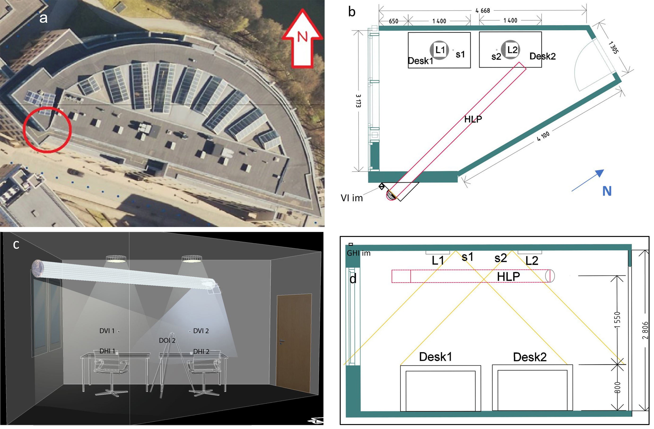
Fig. 1. Full-scale test office. (a) Situation plan of the Norconsult Headquarters in Sandvika; (b) plan of the test office, VI im is the outdoor vertical illuminance meter; (c) model of the office with sources of illumination: window, HLP, and luminaires; position of the five indoor illuminance meters is indicated with DHI 1, DVI 1, DHI 2, DVI 2 and DOI 2; (d) section of the room, Desk 1 is closest to the window and desk 2 is closest to the door. The HLP exit is near the desk 2 and the custom-designed reflector direct the daylight to the desk 2. Desk 1 is to be lit by artificial lighting from luminaire 1 (L1), and desk 2 from luminaire 2 (L2). S1 is the DLC sensor connected to L1, and S2 is the sensor connected to L2. GHI im is the outdoor illuminance meter on the roof.
2.1.2. Sun-shading strategy in the test office
The sun-shading strategy was developed in the test office to provide visual comfort at any time of the day and year, thus creating a glare-free space that would be reliable for the estimation of energy consumption and saving. The sun-shading strategy in the office consisted of keeping the outdoor sun-shading slats, which were manually controlled, partly open at a tilt angle 45°, which is the sunlight cut-off angle at the location. The glare-free space ensured that situations with excessive sunlight would not occur at all, and the users’ need to close the blinds would be completely prevented. Figure 2 presents the view toward the window from the entrance of the office (2a), from Desk 2 (2b), and from Desk 1 (2c).
Figure 2
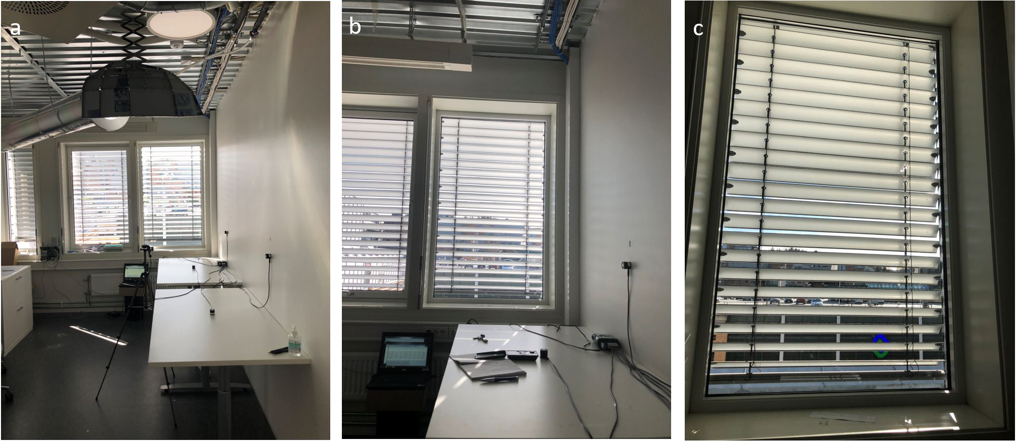
Fig. 2. The view against the window and potential for excessive sunlight and glare: from the entrance to the office (a); from the desk 2, closest to the door (b); from the desk 1, closest to the window (c).
The outdoor venetian blinds had curved slats (8 cm width and 1 cm thick) and were positioned within a frame. The distance between slats was 8 cm. The sun-shading slats were made of semi-specular white aluminium. The configuration of the slats’ angle (partly open at a tilt angle 45° for a sunlight cut-off) was based on the study by T. Kolås [10] that was performed for the same location as the present study.
2.1.3. Daylighting conditions in the office
Daylight in the office was provided by two windows facing southwest. The daylight calculations (using Dialux 4.3 software) for the room were performed by applying the aforementioned sun-shading strategy (section 2.1.2) to check what would be reasonable to expect for the daylight supplementation on the two desks in the office. These calculations were done without accounting for the daylight from the HLP. Results were reported in the appendix A1 in the qualitative part of this full-scale study which was recently published [2]. Under a clear, sunny sky, without direct sunlight (with approx. outdoor illuminance 15 Klx) during equinox at 12:00 h (sun’s altitude of 30°, azimuth of 180°), the values would be 350 lx on the desk 1, closest to the window, and 120 lx on the desk 2, closest to the door.
2.1.4. Horizontal light pipe in the test office
The HLP used in this study was the LW300 manufactured by the producer LightWay. Due to the building’s constructive issues, the maximum diameter of a pipe that could be applied was 22 cm. Dictated by the aim of the study, to have a pipe’s exit near the desk 2, the necessary length of the pipe was 375 cm. These dimensions provided an aspect ratio of the installed light pipe of 17, which corresponded to a semi-empirical study recently done by the authors [1]. The reflection factor of the inner surface of the pipe is 99.8% according to the manufacturer. The light pipe’s dome had a diameter of 26 cm, was manufactured out of crystal glass, and had a light transmission factor of about 95% (test performed by the authors) (Fig. 3(a)). The light distributor, that is the element of the light pipe that releases the light into the indoor space, was chosen to be clear glass with a light transmission factor of 92%. The direction of the light onto the working area was provided by a custom-made reflector, thus using the same approach as in the semi-empirical study recently done by the authors [1]. Here, the aim was to redirect the light to the working area (desk 2 and the wall in front of it) while maintaining the qualitative features of the daylight e.g., dynamics, variation, light patches and colour, which are possible to deliver through the HLP.
Figure 3
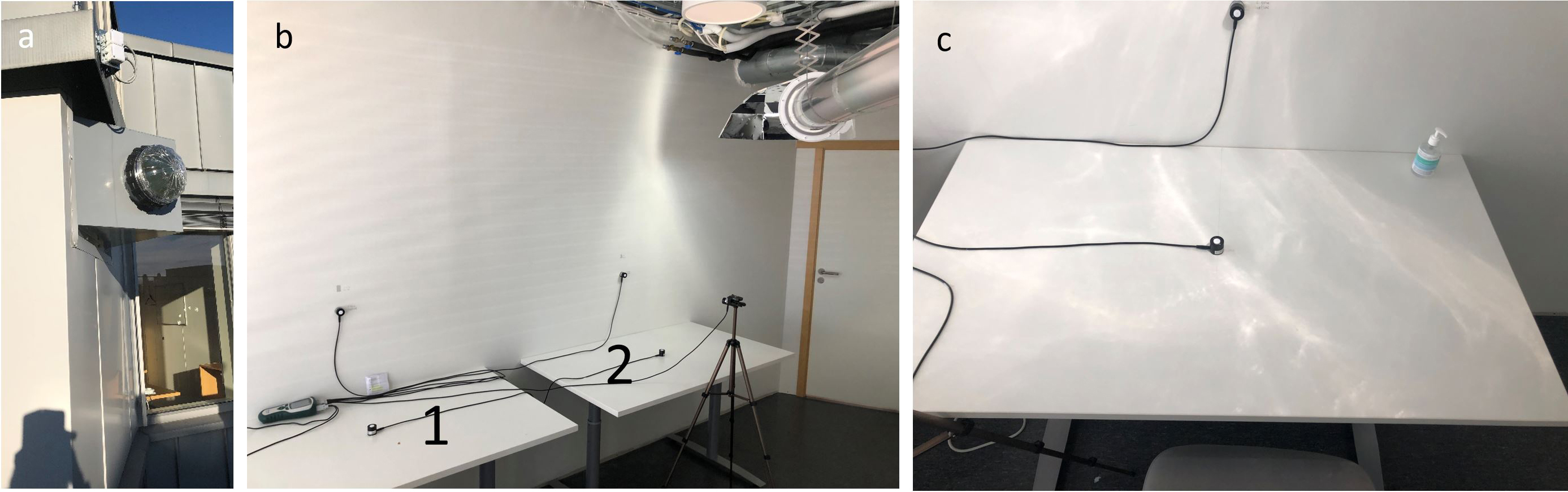
Fig. 3. Light pipe’s dome mounted on the façade (a); light pipe’s exit in the room with custom-made reflector, and two working areas in the room, Desk 1 and Desk 2 (partly leakage of the daylight from the pipe’s exit is visible on the wall) (b); daylight and light patches on desk 2 delivered from the HLP and via a custom-made reflector (c).
The design of the custom-made reflector underwent several stages. Due to the scope of this paper just a brief description is provided. After the HLP was installed (winter 2019), the light output pattern visible on the wall adjacent to the pipe’s exit was observed to understand the expected light distribution at different times of the day and the year. It was first observed that the light flux leaving the tube is concentrated in a circular belt around the edges of the tube (Fig. 4(a)). The angle of the outcoming light rays from the HLP (a cone distribution) was found to be suitable for use of a concave mirror (a custom-made reflector) to obtain the supposed light coverage on the imaginary surface (desk 2 and part of the wall in front of it, Appendix C). The optimal shape of the reflector would be a parabolic-formed continuous 3D-surface, as discussed by J. Chaves [40]. Due to limited budget the reflector had to be composed of flat and assembled mirror surfaces. To keep the number of reflector surfaces as low as possible, it was decided to divide the reflector into a grid of 4 X 4 parts. The multimirror consisting of 16 surfaces, was possible to construct with simple workshop conditions while keeping the manufacturing error and cost low (Fig. 4(c)). The limitation of the reflector design lies in the free height of the room, which was necessary to account for. This resulted in a shorter reflector on the bottom, and consequently, the daylight coming from the lower part of the pipe was not directed down onto the desk. The reflector was designed using 3D Autocad software and handcrafted out of lightweight aluminium sheets and manually layered by 3M-mirror folium with a 99% light reflectivity.
Figure 4
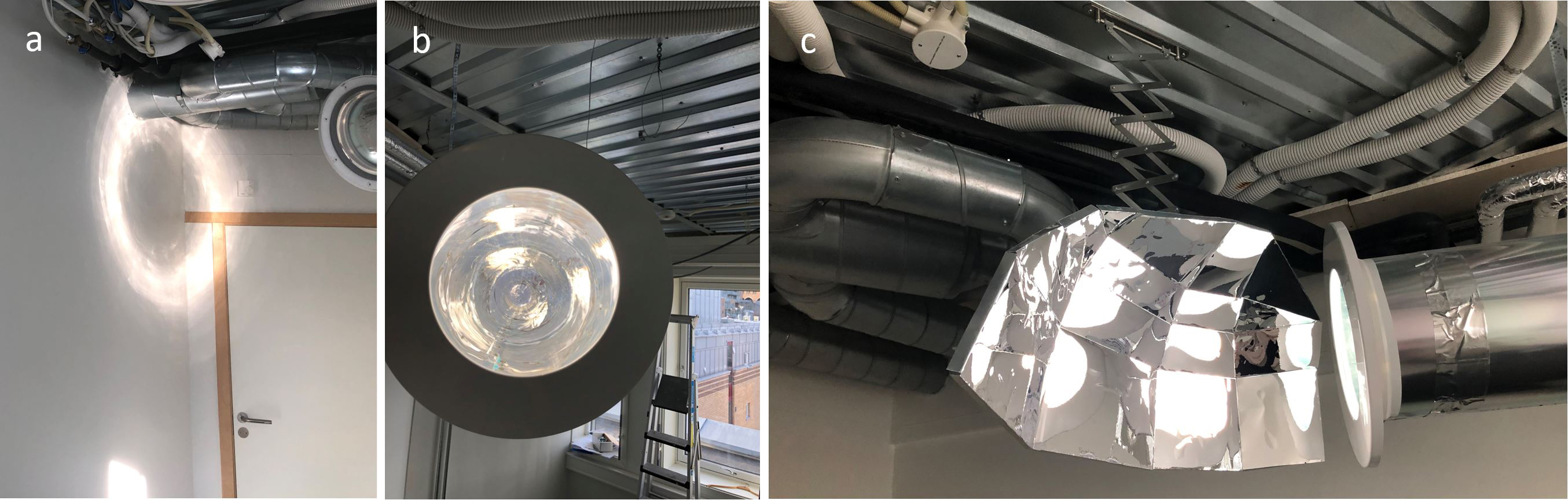
Fig. 4. Circular belt formed by light output from the HLP with clear transparent diffuser on the adjacent wall (2 m-distance) in January at noon (a); view of the light pipe opening, with mirror surface (b); custom-made reflector; the suspension is enabled by a scissor mechanism that allows for an easy adjustment in place (c).
All reflected rays, predicted upon the design, fall within an area up to 1.2 m from the centre of the table and spread over the imaginary circular task surface which covers the table and the wall in front of it (Appendix C). However, the ad hoc measurement performed during the equinox, with darkened windows, to check the reflector performance, revealed that the daylight is spread also on the desk 1 (Fig. 5). This could have happened due to the white colour of the desk 2 and light colour of walls which contributed to effective spread of light in the room by interreflections. Between 200 and 300 lx is recorded by the three sensors assigned to the desk 2 and up to 50 lx on the 2 sensors assigned to the desk 1. The weather was clear and sunny and the maximum vertical illuminance incident on the HLP was between 60-80Klx.
Figure 5

Fig. 5. Recorded values for the daylight illuminance provided just by HLP with the custom-designed reflector, during three days around equinox. Desks 1 or 2 refer to the desk closest to the window and the desk far from the window, respectively. The illuminance is measured horizontally and vertically for both desks, and, the last point, horizontally, between the two desks.
2.1.5. Electric lighting in the office
The electric lighting in the test office was designed according to the Norwegian best practice to ensure fulfilment of lighting recommendation. Lighting solution consisted of two smaller, ceiling-mounted luminaires, manufactured by Glamox. The luminaires provided 2700 lm each, which enabled the required 500 lx of horizontal illuminance on both desks along with a uniformity of over 0.6, as specified in NS-EN 12464-1 (standard for illumination for indoor workplaces). The luminaires had a colour temperature of 4000 K and a colour rendering of Ra = 80.
The estimated LENI, using Dialux 4.13 software, was 10.37 kWh/m2year. The calculation was based on a seven-day week and ten hours of occupancy, where just daylight dependency factors were employed. The operational hours of electric lighting based on the availability of usable daylight were counted based on the threshold of solar altitude over 5° and accounting for the sun-shading on the windows as well (Appendix A). The daylight time usage was set to 2524 hours and non-daylight time usage was set to 1116 hours which in total results in 3640hours. Each luminaire was connected to a separate photosensor and programmed by a DLC. Luminaires should supplement with additional light when the daylight provided by the windows and light pipe does not reach 500 lx.
When lighting scheme consists of more than one luminaire there is an ‘overlapping’ illuminance effect. For example, one luminaire is able to provide 440 lx on the desk below it and up to 150 lx on the other desk (in the middle point of each desk). The effect is totally equal for both luminaires, as they are identical and have equally located in relation to the desks. As luminaires are controlled separately the energy use for each of them will be different, hence the provided illuminance solely from the electric lighting must be estimated considering the overlapping effect. Figure 6 shows the relation between the power (energy consumption) and illuminance on the desk under, as well as that supplemented to the other desk. The luminaire closest to the window is referred here to as ‘L1’, and the luminaire closest to the door is referred to as ‘L2’.
Figure 6

Fig. 6. Correlation between electric lighting power of each luminaire and the illuminance level on the desk under it or supplemented to the other desk. The effect is equal for both luminaires.
2.1.6. Daylight and electric lighting control system
The system was calibrated during the night (i.e., without daylight in the room), and the established controlling was with a 10-minute fade time from maximum to minimum flux, based on a measuring value of the last 1 minute, for each desk separately. This corresponds to the best practice in Norway, which is based on the experience with characteristic daylighting conditions. Applying this approach for DLC sudden peaks and drops in the light were avoided, as this would have otherwise disturbed the occupants. The qualitative part of the study discusses and proves this finding [2]. The DLC components used in this study were ‘off-the-shelf’ products. This means that the results of this study are based on the use of products available on the market during the study period. Further, this acknowledges the limitation of this study, that the results could be different if this study (or a future similar one) had applied a different DLC strategy (i.e., choosing an alternative photosensor type or controlling algorithm).
The photosensors used for this DLC system, manufactured by Glamox, had a wide angle (120°, bicubic) and lacked any shield in order to obtain information on a wider field (where the daylight from the HLP was intended to be directed). The sensors were slightly tilted toward the wall (10°), as discussed in the introduction, so that the visual field could measure the vertical illuminance on the wall as well. The decision of photosensor position was made in order to detect differences in the illuminance values on both of the desks individually and to correlate these values with the supplementary illuminance the luminaires supposed to provide. The sensors were positioned near each other (Fig. 1) according to the most common practice with two working places, but this proximity was not closer than in the case of using a luminaire with an integrated sensor. In a case when both sensors are positioned too close to the window, they are assumed to not be affected by the excessive daylight on the working areas due to the sun-shading strategy applied. However, the authors did not predict that the light reflected on the slats—at a given tilt—would be redirected directly to the sensor.
2.2. Monitoring procedure and measuring equipment
The monitoring procedure included measuring the indoor illuminance, outdoor illuminance, and energy consumption of the electric lighting every minute from 7am to 17pm, which was referred to as ‘occupancy hours’ in this study. Parametric measurements were logged continually on a PC. To ensure the study quality, standard calibrated measuring equipment was used.
Monitoring of the indoor illuminance was performed using 5 Ahlborn illuminance meters FL623VL and an Almemo logger to log the data on the PC. The illuminance meters were positioned to cover the horizontal illuminance on the desk closest to the window (desk 1, DHI 1) and the desk closest to the door (desk 2, DHI 2) at the 0.8 m height, then, the vertical illuminance on the wall in front of both work areas (DVI 1 and DVI 2) at the 1.2 m height). The last illuminance meter was positioned on a tripod to record the vertical illuminance at the eye level of the user of desk 2 (DOI 2). The position of illuminance meters is illustrated in Fig. 1(c). The CIE recommendation of using grid points is related to ad hoc point measurements, while using only one illuminance meter per desk is recommended for continuous measurements, as argued by T. Kruisselbrink et al. [41] and N. Gentile et al. [42]. Illuminance meters in this study were placed at a location critical to or representing the typical illuminance of that zone. A placement of photosensor coinciding with the luminaire position is not recommended, but, in this project, the same place is the target for the output of the daylight via the HLP; therefore, the place was assumed as the most suitable position. Monitoring of the outdoor illuminance was performed via photosensors (Carlo Gavazzi lux sensors BSH-LUX-U) placed vertically along the same south-oriented vertical plane as the tube’s entrance dome (Figs. 1(b) and 7(a), marked as VI im), to measure vertical illuminance (VI) as well as via photosensors placed horizontally on the roof of the building (Figs. 1(d) and 7(b), marked as GHI im) to measure global horizontal illuminance (GHI). The measurement data was retrieved via a monitoring software UPW3 tool developed by Carlo Gavazzi. The lighting energy consumption was measured using separate power meters (10–20 A) for each luminaire. The scheme for electric lighting solution and monitoring equipment for lighting energy use is presented in Fig. 8.
Figure 7
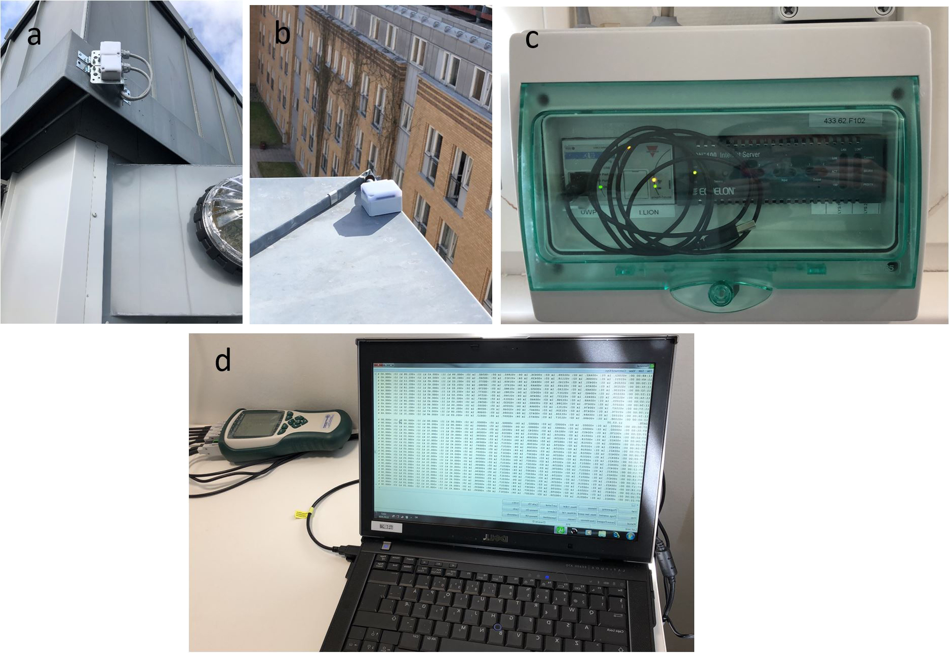
Fig. 7. Monitoring equipment: (a) Monitoring of the VI incident on the HLP, VI im; (b) monitoring of the GHI, GHI im; (c) logging of energy consumption of each luminaire; (d) logging of the indoor illuminance measurements from the five illuminance meters.
Figure 8
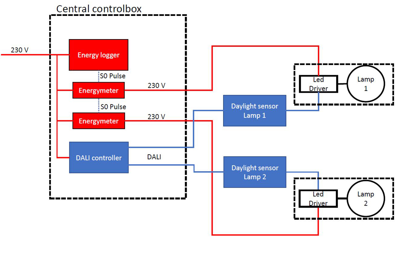
Fig. 8. Scheme for electric lighting solution in the test office and monitoring equipment for electric lighting energy-use.
3. Monitoring results and analyses
Prior to analyses, it is necessary to note some facts the researchers became aware of just prior to the start of the monitoring period. It has been noticed that the daylight conditions during the test and reference periods were not completely equivalent. Daylighting conditions are the only independent conditions (input data) that all other conditions (here, electric lighting and energy consumption) depend on. According to Satel-Light database (measured for the years 1996–2001), the global illuminance data for Oslo reveals that there are higher values for the spring period of each year compared to the autumn (Appendix B1). The difference in weather conditions (and daylight illuminance values) affects the lighting energy use during the test and reference monitoring period. The authors’ perspective is that the validity of the results of this study is the important issue; they therefore chose the test period of the study to be during the worst conditions (lower daylight values), as this would represent the most reliable results.
In order to compare recorded values for the outdoor and indoor illuminances, pairs of days for test and reference period were chosen, Fig. 9. The days for each pair have compatible independent variables (equal solar altitude and profile of daylight conditions (values excluding VI and GHI during the day)), which establishes the validity of the analyses, and the reliability of the data being compared.
Figure 9
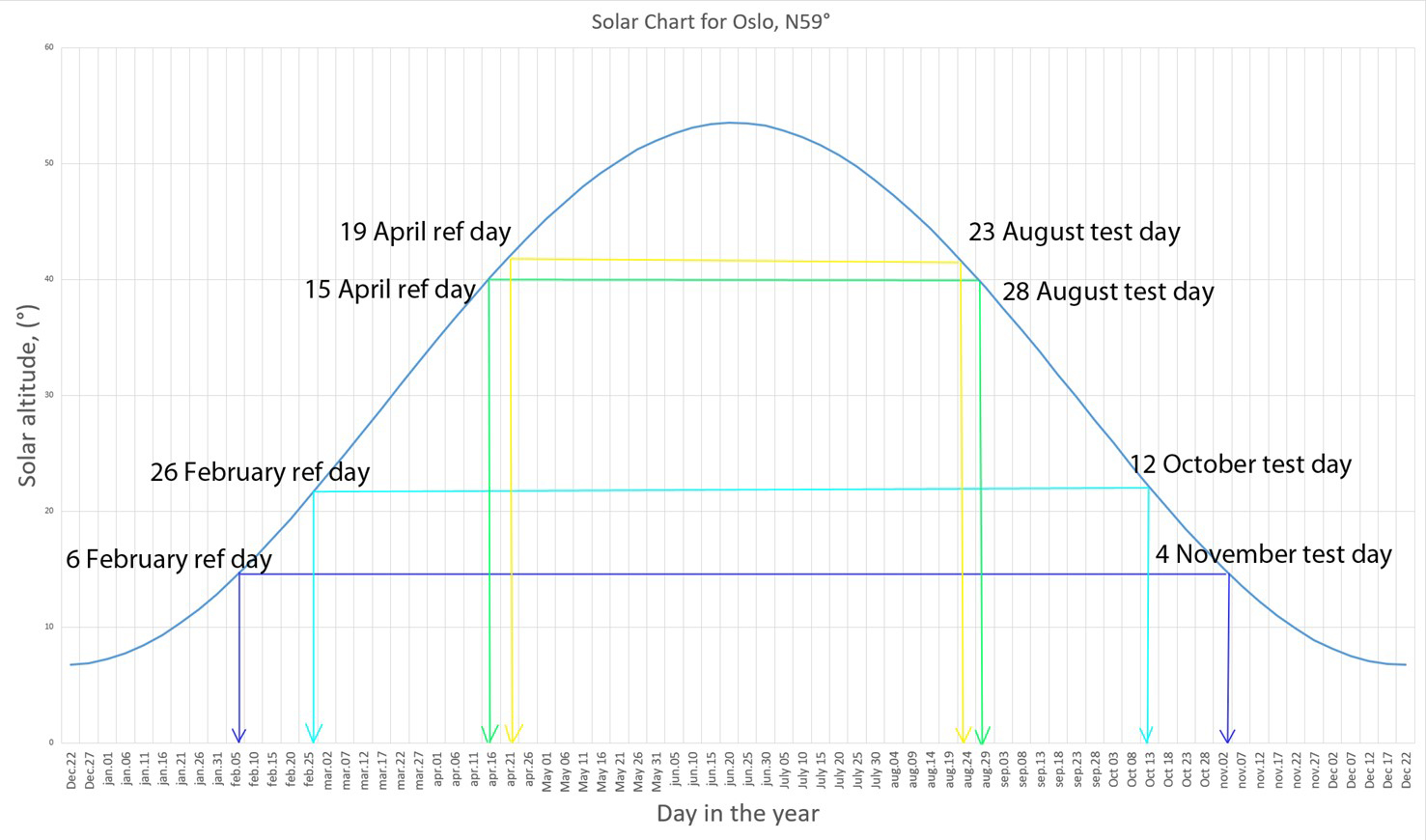
Fig. 9. Solar altitude compatibility for test and reference pair of days used in statistical analyses.
As daylight supplement via HLP (and a custom-designed reflector), directed to the working area, is not uniform (caustic effect is visible in the Fig. 2(c)) analysing a single point value could be unreliable. Recorded data from all 3 sensors assigned to the desk 2 (on the desk (DHI 2), on the wall (DVI 2) and on the observer’s position (DOI 2)) can be used to discuss the values of the daylight on the spread task area. In addition, the effect of the daylight via HLP, on the desk 1, is also present, as described in the section 2.1.4. Hence, the two illuminance meters assigned to the desk 1 could be used in the discussion as well. Thus, the outdoor vertical illuminance (VI) was assumed to have a direct influence on desk 2 as the daylight via HLP is directed at it, and to a smaller extent on desk 1; while global horizontal illuminance (GHI) supplemented through the window, is assumed to have higher influence on desk 1, and lower on desk 2.
In order to analyse the supplement of HLP (with the reflector), illuminance values recorded on all five illuminance meters when electric lighting was dimmed down to zero should be considered. During clear and sunny sky condition dimming of the electric lighting totally to a zero-value occurred around the noon, even when the illuminance measured by the DLC sensors did not reach the threshold value of 500lx. The authors discovered that the major reason for this was the daylight reflection on the semi-specular sun-shading slats (at a tilt angle 45°, for sunlight cut-off), resulting in a partial re-direction of the light to the DLC sensors. As such, the luminaires often received incorrect information regarding the supplementary illuminance they needed to provide, which resulted with lower illuminance values (which was recorded by the illuminance meters) then the threshold.
In Fig. 10, an example of the recorded values of the outdoor (VI and GHI), and indoor (DHI 1, DVI 1, DHI 2, DVI 2 and DOI 2) illuminance for the test and reference pair days is presented for the time with luminaires dimmed down to zero (between 12:00am and 14:30pm). During the time with close to equal outdoor daylight conditions (blue and orange areas in the graphs) recorded values on the three sensors on the desk 2 (red, orange, and yellow lines) are much higher for the test day than for the reference day.
Figure 10
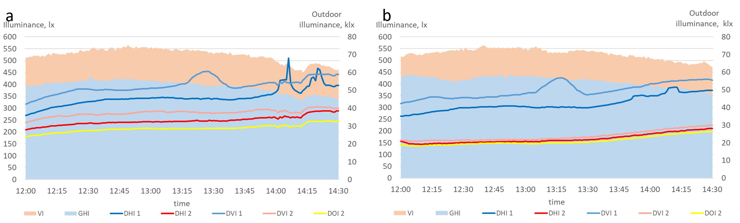
Fig. 10. Aggregative graphs of the illuminance values recorded for the test (a) and reference (b) pair days which were recorded between 12:00am and 14:30pm. The light orange area presents vertical illuminance incident on the pipe (VI), while light blue area presents global horizontal illuminance (GHI); Bluish lines present illuminances recorded for the desk 1, and red, orange and yellow lines present illuminance values recorded for the desk 2.
The scatter plots in Fig. 11 illustrate the relation between illuminance values recorded on all sensors with the vertical illuminance incident on the pipe (VI). For the same VI values (horizontal axis) the illuminances measured by all illuminance meters show higher values for the test day than for the reference day.
Figure 11
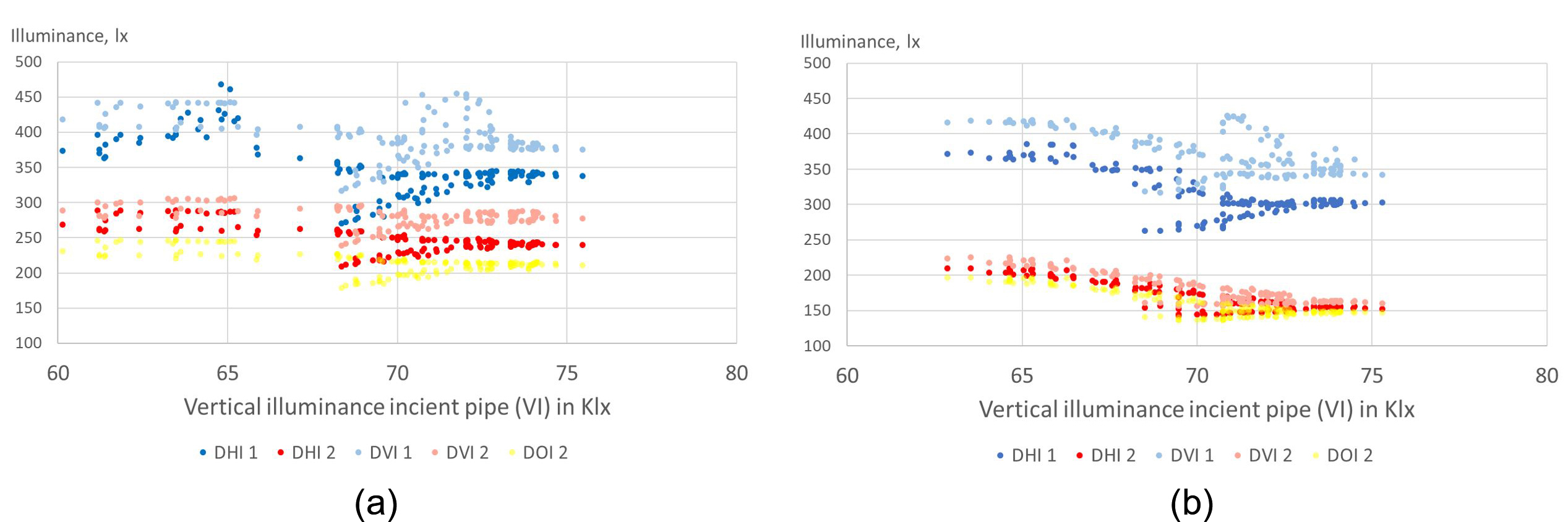
Fig. 11. Illuminance values for the test (a) and reference (b) pair days which were recorded between 12:00am and 14:30pm. The scatters show the illuminance values recorded for all five illuminance meters referred to the vertical illuminance (VI); Bluish lines present illuminance recorded for the desk 1 and red, orange and yellow lines present illuminance values recorded for the desk 2.
3.1. Statistical analyses of photometry recordings
In order to answer research questions in this study, inferential statistical analyses were used to test hypotheses placed at the beginning. Hence, the analyses checked if the recorded values for DHI 1, DVI 1, DHI 2, DVI 2 and DOI 2 are higher in the case of test days compared with the reference days. Figure 9 presents the pair of days for test and reference period (chosen to cover the equal daylight profiles) used in the analyses. To performed statistical analyses just a period (each minute recorded values) when electric lighting is dimmed to 0 is taken in comparison. This period is between 12:00am and 14:30pm. In the following Tables independent sample t-tests (with following graphs) and a point biserial correlation (PBC) are shown. The IBM SPSS 27 software was used to performed statistical analyses. Bonferroni correction, usually used to account for error type 1, in large sample size analyses, was not used, simply because of the nature of values in population samples. The variables in the analyses are the values of external and internal illuminance, which in the entire population can vary greatly, (due to the sudden passage of clouds and the covering of the sun, or due to the intensity of the illumination recorded on the indoor light meters), and these situations were exactly something that the analyses should not have taken into consideration.
Independent t-test is used to compare Mean values of the independent variables (VI and GHI) with the Mean values of the dependent variables (DHI 1, DVI 1, DHI 2, DVI 2 and DOI 2) and to draw a picture about the effect of the HLP presence during the test days. Difference presented in the figures following tables shows relative difference between Mean values of test and reference days (Test-Ref)/Ref), thus showing the improvement (in %) for the test comparing to the Ref.
In the point biserial correlation analyses, all dependent variables (DHI 1, DVI 1, DHI 2, DVI 2 and DOI 2) are used in corelation with binary nominal explanatory variable (test = 1 and reference = 0) to get the value of correlation coefficient. The result of biserial correlation is a coefficient R which is used to build a relation between the variables. The relation (R2) is presented in the graphs following tables (for solely DHI 2 and DVI 2).
First pair of days is the test day 4 November 2020, and the reference day 6 February 2021. Table 1 presents independent sample t-test analysis. Mean values of VI and GHI for test and reference days are nearly equal (44.92 Klx and 44.28 Klx for the VI, and 5.09 Klx and 4.95 Klx for the GHI, for test and reference day respectively), but the recorded indoor illuminance values for the test and reference day show statistically significant difference (p = <.01) for all parameters. Figure 12 presents comparison of Mean values resulting from the independent t-test analyses. Relative difference of Mean values for DHI 2 and DOI 2 is slightly under 40% for test day comparing to the reference day. Moreover, relative difference of Mean values for DVI 2 is over 70%, meaning that the DVI 2 value were 70% higher in case of test day compared to the reference day.
Table 1
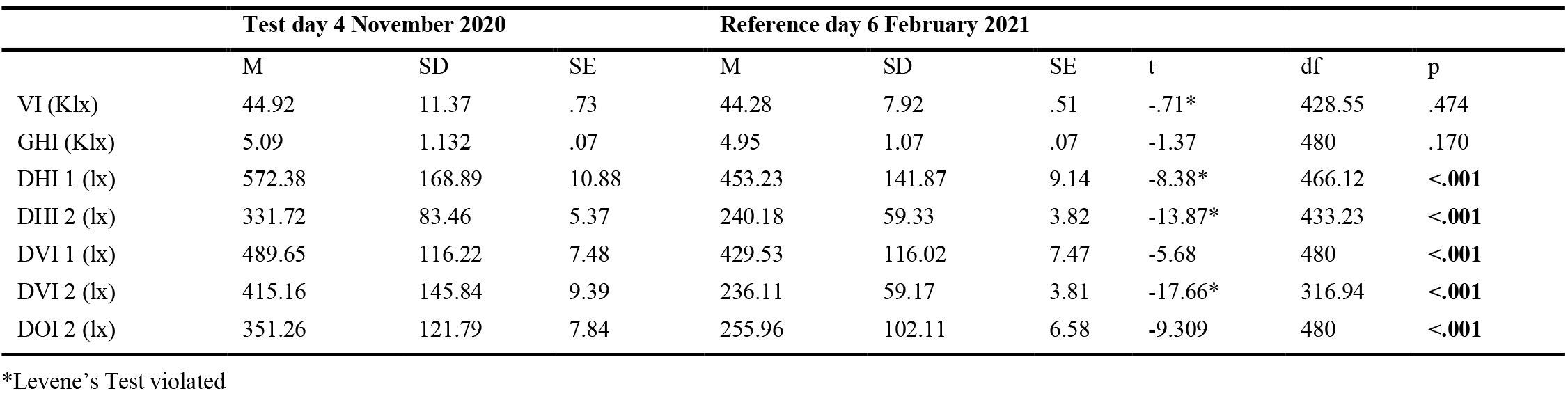
Table 1. Independent sample t-test analysis compares mean values for independent and dependent variables for test day 4 November 2020 and reference day 6 February 2021.
Figure 12
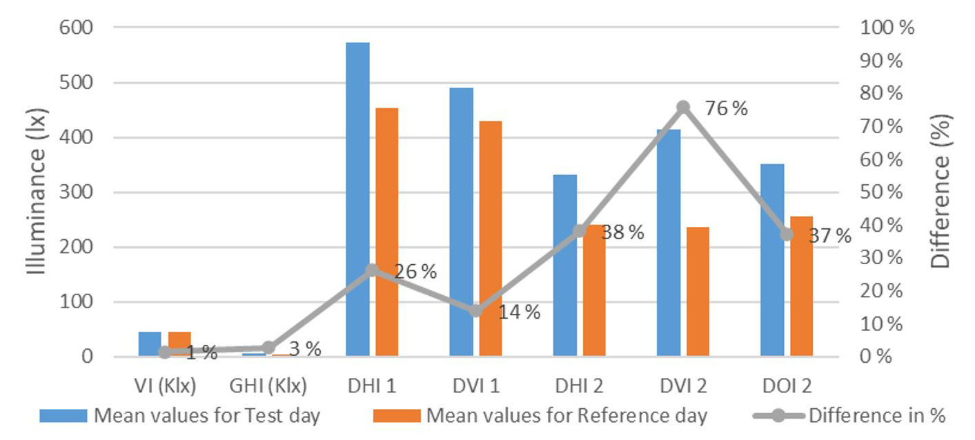
Fig. 12. Comparison of Mean Illuminance values for the test and reference pair days which were recorded between 12:00am and 14:30pm. VI and GHI are shown in Klx.
In Table 2, Point bi-serial correlation test for all independent (VI and GHI) and dependent variables (DHI 1, DVI 1, DHI 2, DVI 2 and DOI 2) shows correlation strength regarding increase of the nominal parameter (0 for ref and 1 for test). Statistically significant correlation (p<.01) is shown for all dependent variables, meaning that the values were higher for the test day (nominal parameter 1). The PBC coefficient (R2) is higher for the DHI 2 (.535) and DVI 2 (.628), which is also illustrated in Fig. 13.
Table 2
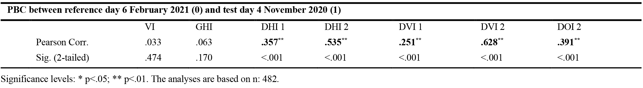
Table 2. Point bi-serial correlation test for the test day 4 November 2020 and reference day 6 February 2021.
Figure 13
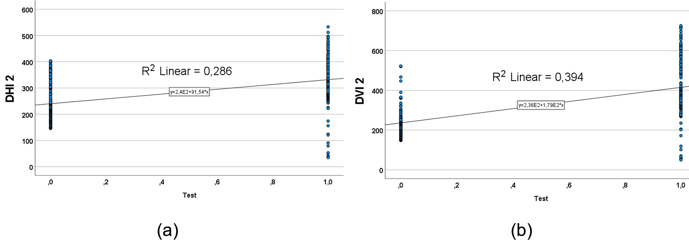
Fig. 13. Point-biserial correlation coefficients show a relation between the values of DHI 2 (a), and DVI 2 (b) for pair of days, reference (0) and the test (1).
Second pair of days is the test day 12 October 2020, and the reference day 26 February 2021. Table 3 presents independent sample t-test analysis for this pair. Mean values of VI for test and reference days are 65.33 Klx and 71.02 Klx, respectively. Mean values of GHI for test and reference days are 16.19 Klx and 11.73 Klx, respectively. Thus, this pair of days has slightly lower VI and higher GHI values for test day compared with reference day. Recorded indoor illuminance values for the test and reference day show statistically significant difference (p = <.01) for all parameters. Figure 14 presents comparison of Mean values resulting from the independent t-test analyses. Relative difference of Mean values for DHI 2 and DVI 2 is over 100%, meaning that the values were two times higher for test day comparing to the reference day. The relative difference of Mean value for DOI 2 is 70% in case of test day comparing to the reference day.
Table 3
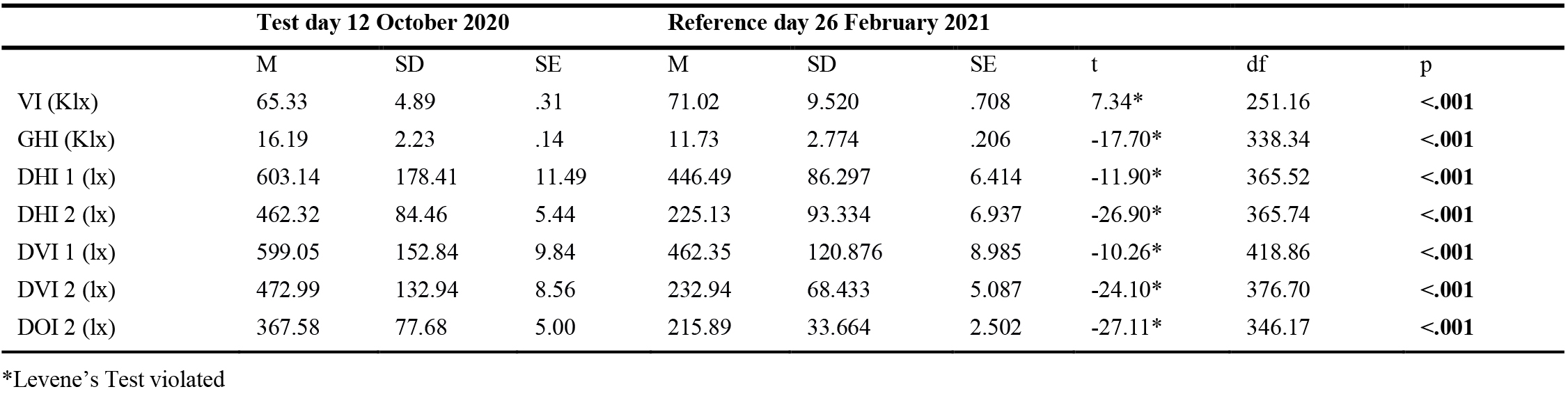
Table 3. Independent sample t-test analysis compares mean values for independent and dependent variables for test day 12 October 2020 and reference day 26 February 2021.
Figure 14
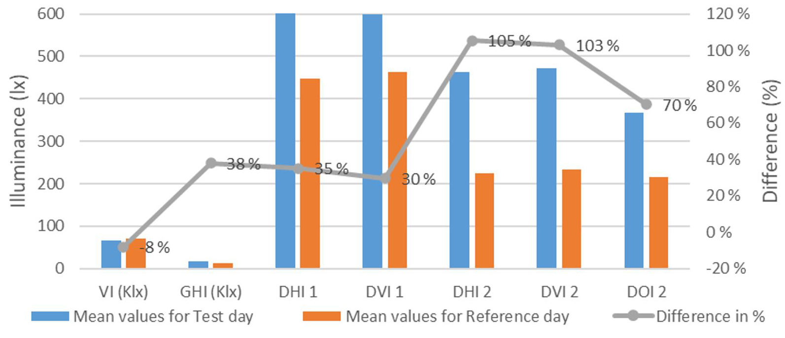
Fig. 14. Comparison of Mean Illuminance values for the test and reference pair days which were recorded between 12:00am and 14:30pm. VI and GHI are shown in Klx.
In Table 4, point bi-serial correlation test for all independent (VI and GHI) and dependent variables (DHI 1, DVI 1, DHI 2, DVI 2 and DOI 2) shows correlation strength based on the increase of the nominal parameter (0 for reference and 1 for the test). Statistically significant correlation (p<.01) is shown for all dependent variables, meaning that the values were higher for test day (nominal parameter 1). The PBC coefficient (R2) is higher for DHI 2 (.800), DVI 2 (.734), and DOI 2 (.768), which is also illustrated in Fig. 15.
Table 4
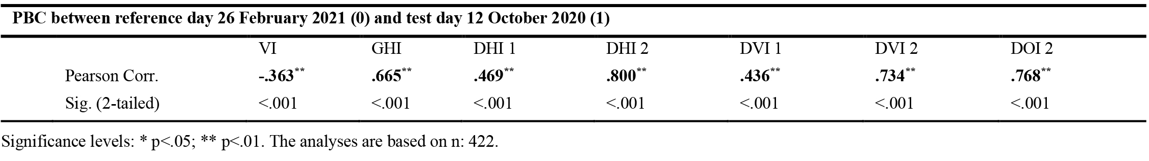
Table 4. Point bi-serial correlation test for the test day 12 October 2020 and reference day 26 February 2021.
Figure 15
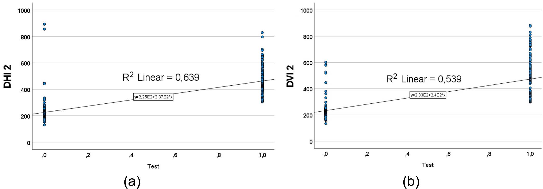
Fig. 15. Point-biserial correlation coefficients show a relation between the values of DHI 2 (a), and DVI 2 (b) for pair of days, reference (0) and the test (1).
Third pair of days is the test day 28 August 2020, and the reference day 15 April 2021. Table 5 presents independent sample t-test analysis for this pair. Mean values of VI for test and reference days are 71.40 Klx and 66.63 Klx, respectively. Mean values of GHI for test and reference days are 48.01 Klx and 50.63 Klx, respectively. Thus, this pair of days has slightly higher VI and lower GHI values for test day compared with reference day. Recorded indoor illuminance values for the test and reference day show statistically significant difference (p = <.01) for all three parameters regarding Desk 2. Figure 16 presents comparison of Mean values resulting from the independent t-test analysis. Here, the relative difference of Mean values for DVI 2 is over 40%, while the relative difference of Mean values for DHI 2 and for DOI 2 is over 30% and over 20%, respectively. This shows the improvement for the test day.
Table 5
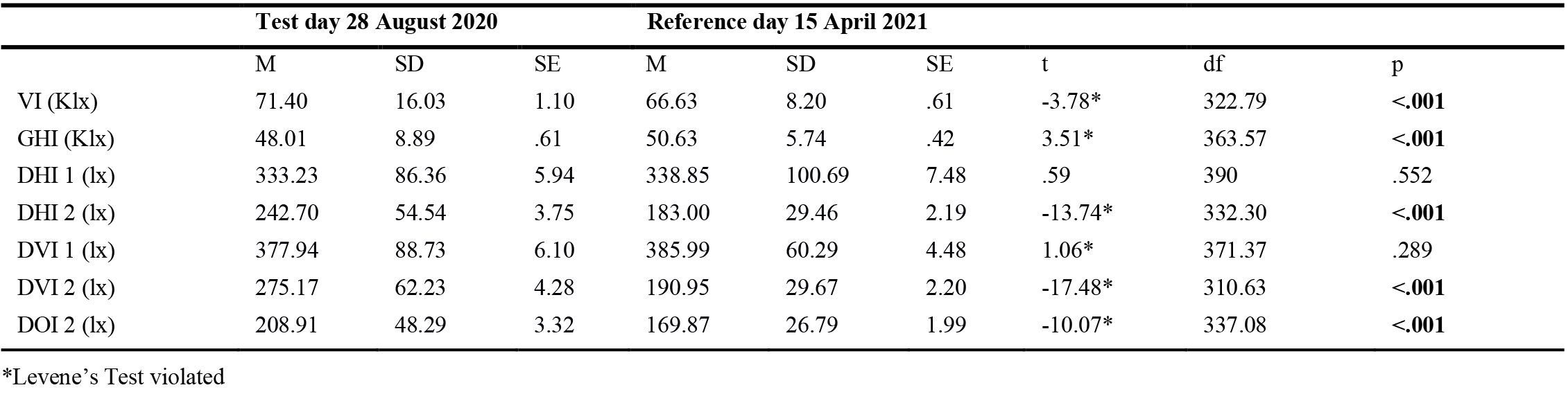
Table 5. Independent sample t-test analysis compares Mean values for independent and dependent variables for test day 28 August 2020, and reference day 15 April 2021.
Figure 16
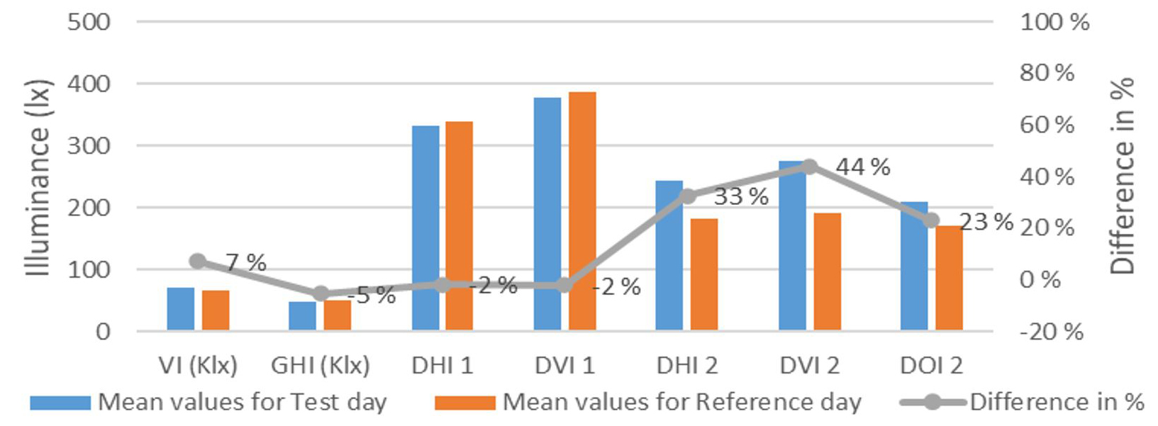
Fig. 16. Comparison of Mean Illuminance values for the test and reference pair days, recorded between 12:00am and 14:30pm. VI and GHI are shown in Klx.
In Table 6, point bi-serial correlation test for all independent (VI and GHI) and dependent variables (DHI 1, DVI 1, DHI 2, DVI 2 and DOI 2) shows correlation strength based on the increase of the nominal parameter (0 for ref and 1 for test). Statistically significant correlation (p<.01) is shown for all dependent variables regarding desk 2, meaning that the values were higher for test day (nominal parameter 1). The PBC coefficients (R2) show positive correlation for the DHI 2 (.555), DVI 2 (.645), and DOI 2 (.440), which is also illustrated in Fig. 17.
Table 6
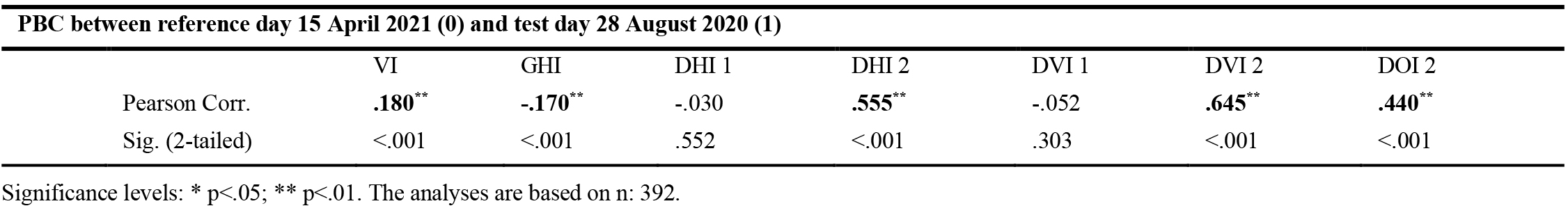
Table 6. Point bi-serial correlation test for the test day28 August 2020, and reference day 15 April 202.
Figure 17
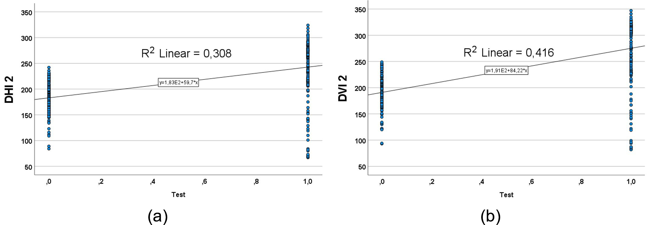
Fig. 17. Point-biserial correlation coefficients show a relation between the values of DHI 2 (a), and DVI 2 (b) for pair of days, reference (0) and the test (1).
The last analysed pair of days is the test day 23 August 2020, and the reference day 19 April 2021. Table 7 presents independent sample t-test analyses for this pair. Mean values of VI for test and reference days are 69.83 Klx and 70.43 Klx, respectively. Mean values of GHI for test and reference days are 52.38 Klx and 54.59 Klx, respectively. This pair of days has nearly equal VI values, while GHI values for test day are slightly lower compared with reference day. Recorded indoor illuminance values for the test and reference day show statistically significant difference (p = <.01) for all parameters. Figure 18 presents comparison of Mean values resulting from the independent t-test analyses. Relative difference of Mean values for DVI 2 is nearly 60%, while for the Mean values for DHI 2 and for DOI 2 is slightly under 50% and over 30%, respectively. This means that the values were higher for the test day.
Table 7
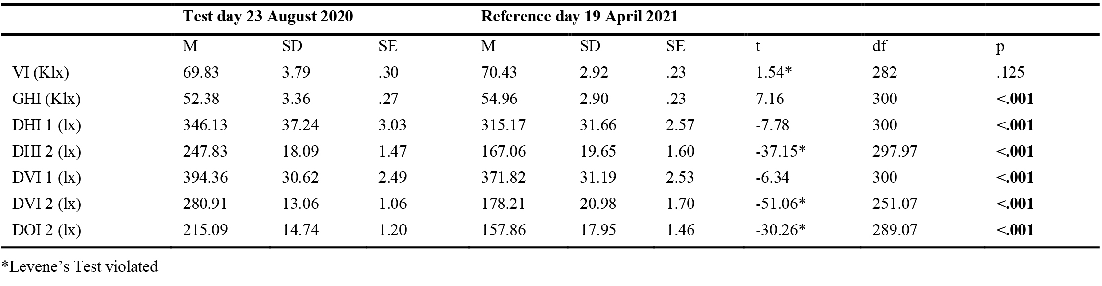
Table 7. Independent sample t-test analysis compares mean values for independent and dependent variables for test day 23 August 2020, and reference day 19 April 2021.
Figure 18
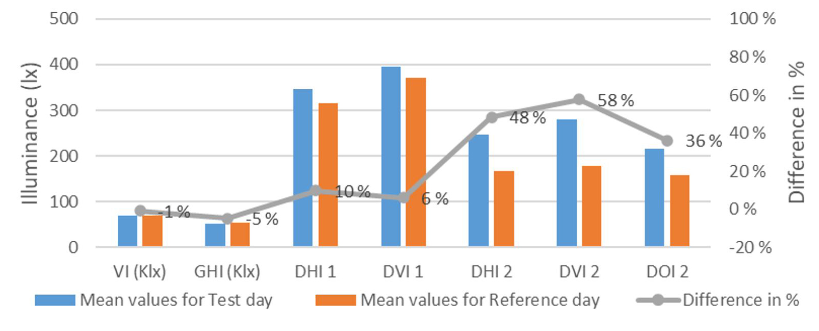
Fig. 18. Comparison of Mean Illuminance values for the test and reference pair days, recorded between 12:00am and 14:30pm. VI and GHI are shown in Klx.
In Table 8, point bi-serial correlation test for all independent (VI and GHI) and dependent variables (DHI 1, DVI 1, DHI 2, DVI 2 and DOI 2) for the test day 23 August 2020 and the reference day 19 April 2021, shows correlation strength regarding increasement of the nominal parameter (0 for ref and 1 for test). Statistically significant correlation (p<.01) is shown for all dependent variables, meaning that the values were higher for test day (nominal parameter 1). The PBC coefficients (R2) show high positive correlation for the DHI 2 (.906), DVI 2 (.947), and DOI 2 (.868), which is also illustrated in Fig. 19.
Table 8
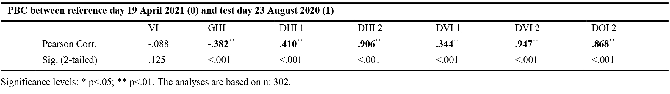
Table 8. Independent sample t-test analysis compares mean values for independent and dependent variables for test day 23 August 2020, and reference day 19 April 2021.
Figure 19
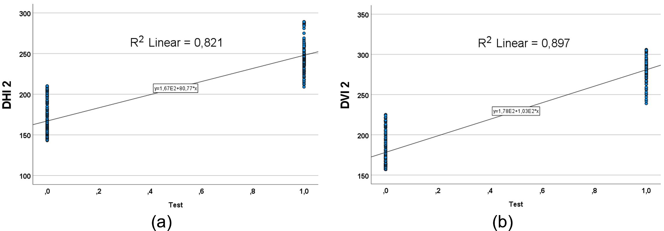
Fig. 19. Point-biserial correlation coefficients show a relation between the values of DHI 2 (a), and DVI 2 (b) for pair of days, reference (0) and the test (1).
Finally, we can answer the research question from the introduction: Does daylighting provision via the HLP leads to an increased level of daylight on the second working area in the office? The recorded data and analyses of pair days demonstrates that, under equal daylighting conditions (here, the sun’s altitude and GHI and VI profiles) the situation with the HLP provides higher illuminance levels on the second task area compared to the situation without the HLP (solely window daylighting). The difference is from 30% to over 100% higher illuminance.
3.2. Lighting energy use and saving potential
The energy-saving potential is an estimate of how much energy can be saved if the original or basic solution is altered with another one. The term energy efficiency is also in use, referring to a practice of using less energy to provide the same amount of useful output from a service or a device. We could talk about the energy efficiency of an alternative luminaire for example, but since this study is about the reduction in energy consumption of a complex solution (a multidevice solution consisting of electric lighting, windows, HLP) the energy-saving potential suits better. The analyses of energy-saving potential in this study rely on the relative difference between the energy used in the reference period and energy used in the test period and is expressed in percentage. The energy-saving potential shows that part of the energy that is used in the base case (reference) and could potentially be saved if an alternative solution were applied.
Monitoring data regarding the energy consumption of both luminaires individually was collected and analysed. The luminaire dimming was found to be linear, as shown in Fig. 6.
The overlapping of the illuminance, as described in section 2.1.5, triggered an unexpected issue, namely the luminaire dominance, that the authors can explain just with reasoning on function of the bus controlling system (DALI), which is not a perfectly coordinated component. It seems that the system has sent signals to each luminaire not at exactly same moment but with seconds of delay. This has been shown to be of great importance to the performance of this lighting solution. Additionally, the signal was sent first to a random luminaire (i.e., not always the same one). Further, the luminaire which turned on first does not only provide lighting onto the desk below but also to the other desk, as argued over (Fig. 6), which then immediately gave information to the photosensor of the ‘delayed’ luminaire about the specific level of illuminance on the desk, giving it the opportunity to provide just the necessary supplementary illuminance to reach the required 500 lx. The result of this occurrence was that the first luminaire took on the role of the dominant illuminance-provider throughout the rest of the day and, consequently, has a much higher energy consumption. This is a consistent and significant occurrence on days with an overcast sky; however, this trend was present under other sky conditions as well.
An analysis of the number of incidents of the dominant luminaire (recorded data) at the beginning of the working day (i.e., 7am) is in Fig. 20. During the test period, which is in total 182 days, L1 was dominant 47 days, while L2 was dominant 121 days; the remaining days in the test period both luminaires started at the same point of time. This shows that the L2 was dominant (exhibiting the dominant illuminance) 2.57 (121/47) times more often than L1. In the reference period (182 days as well), L1 was dominant 66 days, while L2 was dominant 79 days. This results in 1.22 times of L2 as the dominant luminaire comparing to L1. The ratio values showed no correlation with either the winter or summer period, with the daylight effect from the window have potentially been a main reason for this. The assemblage of months was equal for the test and reference period when it comes to the daylighting values at the starting time (for the occupancy period starting at 7am) when the luminaires have started. The only conclusion the authors have to offer is that the initial signal was randomly sent and was not affected by the input illuminance values, which the DLC photosensor could have received.
Figure 20
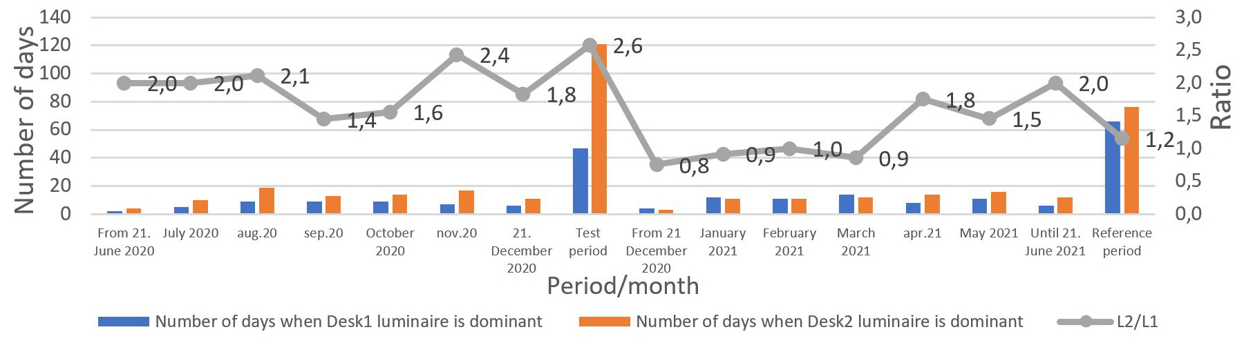
Fig. 20. The number of incidents (days) of one of the luminaires being the dominant light provider for each month in the test period and reference period, and accumulative for test and reference period. A ratio of 1 means that the number of incidents is the same for both luminaires.
As a result, the authors conclude that the collected data on the electric lighting energy use for L1 and L2 in both the test and reference periods was strongly affected by this occurrence of dominant luminaire. Therefore, it was not possible to confidently conclude on the magnitude of the effect this occurrence had on the total energy consumption results for each period, hence the collected monitoring data on lighting energy consumption were concluded as unreliable to be compared.
Authors are not able to answer the research question about the lighting energy saving potential for a single luminaire. However, the authors can report total light energy consumption. The calculated LENI for this test office, was 10.37 kWh/m2year, as mentioned in section 2.1.5, but the value of LENI based on the recorded light energy use for test period of the study was 5.79 kWh/m2year, which can be argued as a direct effect of the daylighting via the HLP. The energy-saving potential could be then expressed as a relative difference between calculated and realistic situation, being ((10.37-5.79)/10.37) 44%. Arguing this we must provide some important notes. The recommended light level (constant and stable target value of minimum 500lx) has not been always achieved in situations when DLC system was affected by daylight reflected from sun-shading, as discussed above. Such situations occurred during the days with clear and sunny sky conditions, which is for the location of this study historically recorded to be about 30% of the daylight time. However, the monitored data and analyses of a pair days suggests that in such situations the illuminance values on the desks were around 400 lx (varying between 300 and 500 lx). This fact indicates that the periods with electric lighting under the recommended level might have contributed to lower energy use.
4. Discussion
After a thoroughly examination of the monitored data, it can be noted that, with similar daylight profiles (i.e., solar altitude, VI and GHI values), the luminaires behaved quite similarly regardless of the illuminance values recorded on the surfaces where the DLC sensors were supposed to look. This indicates that the DLC sensors were affected by the daylight being reflected from the slats during the entire occupancy period. Further, there was only one illuminance meter positioned on each desk recording the illuminance at a point, but there could have been higher illuminance values around this point that the illuminance meter had missed but which the DLC sensors have caught. The lighting patches were of a random nature, as shown in Fig. 3c.
The potential of the HLP to bring about higher daylighting levels has been shown through the analyses in section 3, but there is one more fact to add. Specifically, in this full-scale office, there were glare-free situations, and daylighting via the window was consistently enabled. Such optimal situations cannot be taken for granted in all buildings—even in the newly constructed. On the contrary, it is widely expected that there will be need for sun-shading regulation whenever there is a clear sky and sunlight, and, depending on the sun-shading system, this often will result in total rejection of the daylight via the window. In such situations, the percentage of the daylight supplemented via the HLP, as discussed in chapter 3.1, becomes even more important.
This study shows the potential of a HLP installed on the south façade of unobstructed building at a latitude 60° in increasing the indoor illuminance levels on the horizontal and vertical surfaces positioned at a distance of nearly four meters from the façade. The recorded data and analyses of pair days demonstrate that, under equal daylighting conditions (here, the sun’s altitude and GHI and VI daily profiles), the presence of the HLP results with higher illuminance levels on the task areas compared to the situation without the HLP. An increase in illuminance level on the working area, in the rear part of the office, of approximately 200 to 300 lx, was recorded during clear and sunny days at equinox with HLP enabled and windows darkened. In the same situation HLP provided the increased daylight level on the working area near window of approx. 50 lx. A statistically significant findings from analyses show that at the desk located close to the door, 40% to over 100% higher daylight level can be expected if HLP is used, as compared to the case of solely window-daylighting.
As a consequence of the daylighting via the HLP, the lighting energy-use (justified via LENI) was improved by 44% compared to the estimated value without HLP. This difference in monitored and estimated values is not affected by the occupants’ unpredictable use of sun-shading devices since they have been in fixed setting. This information is of great importance e.g. for on-site energy generation using PV and for ZEB design concepts. Such information is also useful for system capacity decisions, as it can help directly reduce amount of material, costs, and the build-in carbon amount. In the case of ZEN design concepts, it could also provide insight regarding the PV system and the amount of generated energy that will not be needed at the site and that could instead be promised to the energy grid.
5. Conclusion
This full-scale field study resulted in valuable insights into the application of horizontal light pipes (HLP) in office spaces in high latitude areas (Oslo, Norway). In such areas, a low sun angle prevails, and the application of sun-shading devices is critical for the southern, eastern, and western facades of the building. Unfortunately, standard sun-shading devices still operate with a rigid intelligence when it comes to protecting against glare during strong excessive sunlight, reducing the potential for daylight exploitation most of the time. Findings from this study proved that HLP can contribute to a significant increase in the daylight level of the space, both in the rear part, and in the part closest to the window, in cases where the blinds are closed to ensure visual comfort for the users (glare). Furthermore, the novelty in this study, application of the custom-made reflector, contributes to increasing the awareness for daylight distribution inside the space and set the path for future research with daylight transport systems.
The full-scale monitoring revealed some core issues related to unreliable lighting energy forecasting and unmet lighting quality conditions set as recommended illuminance levels on the task surfaces. The decision to apply best practice DLC solution in Norway, without commissioning the solution several times after it was installed, could be seen as one more limitation of this study. The complex relationship between the daylight, sun-shading device, and information-sharing protocols within the DLC system comprise a factor involved in integration failure.
The results from the previously semi-empirical study, using scale model of the HLP, showed that there was potential for improving daylight autonomy (DA) for a HLP of the same aspect ratio (16) and in the same location (Oslo), if laser cut panels (LCPs) were used as a light collector [1,43]. LCP can deflect the incoming light rays to change their propagation angle through the light pipe to a more efficient one. Values of daylight illuminance of up to 300lx, which has been demonstrated in the current full-scale test, can be improved by up to 16%, if a certain LCP configuration described in the semi-empirical study is used. This represents a suggestion for future studies in this field and in high latitude locations.
Appendix A
Figure A1
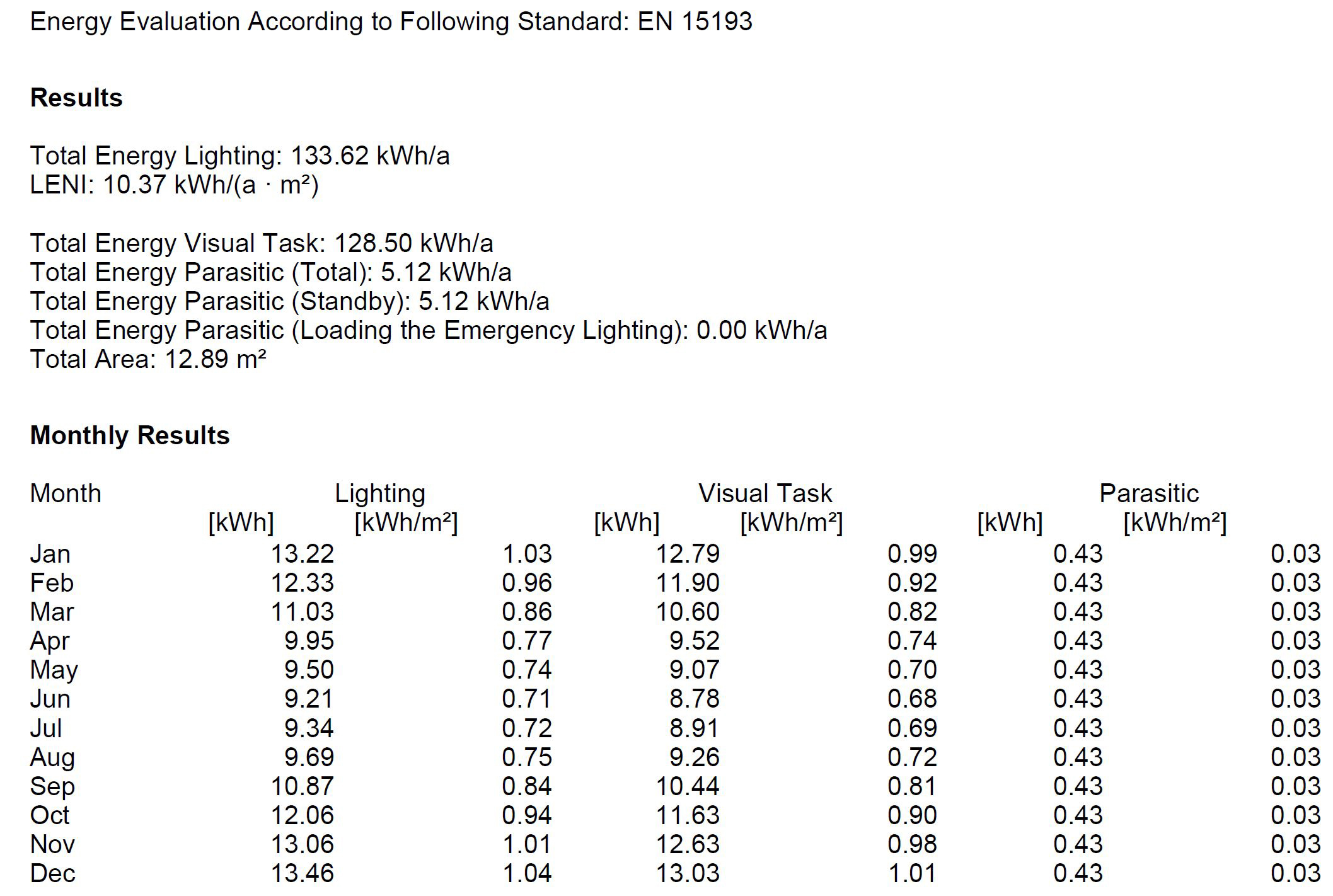
Fig. A1. Calculation of the LENI value for the test office, performed in Dialux 4.13 software.
Figure A2
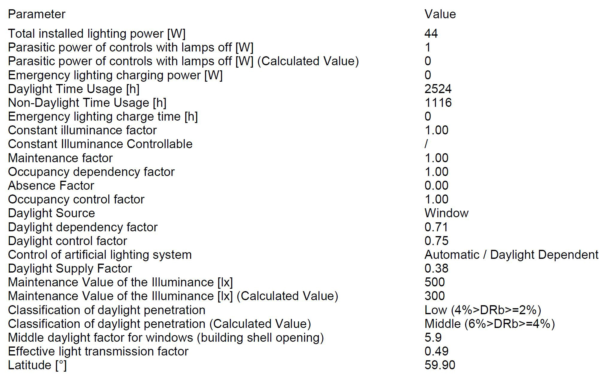
Fig. A2. Parameters used in the calculation of the LENI value for the test office, performed in Dialux 4.13 software.
Appendix B
Figure B1
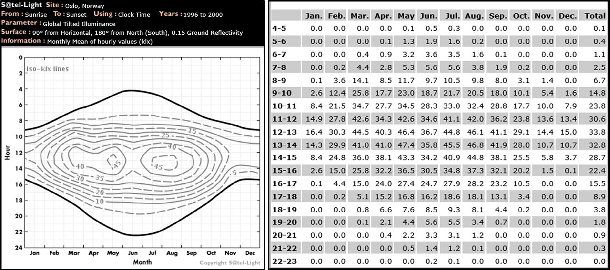
Fig. B1. Global vertical illuminance on the south surface, monthly mean of hourly values. Source: Satel-Light http://www.satel-light.com/pub/Obradovic06052019093340/soutdoor.htm (accessed 20 July 2021).
Appendix C
Figure C1
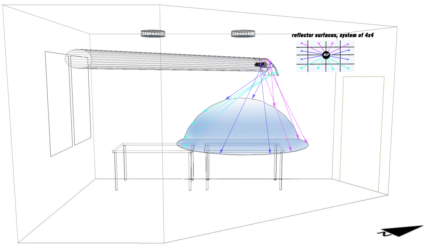
Fig. C1. Side view of 3D model of the test office. A custom-made reflector for HLP light distribution receives the light rays from the HLP and reflects them onto the task surface. The task surface is in the form of a circular plate covering a 1.2 m radius area, including desk 2 and the wall in front of it.
Figure C2
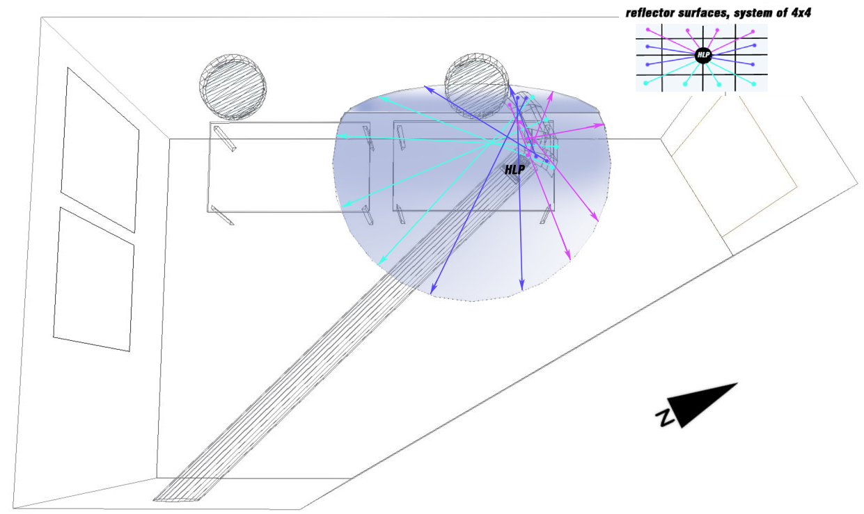
Fig. C2. Top view of 3D model of the test office. A custom-made reflector for HLP light distribution receives the light rays from the HLP and reflects them onto the task surface. The task surface is in the form of a circular plate covering a 1.2 m radius area, including desk 2 and the wall in front of it.
Acknowledgment
This study was conducted as a part of a PhD study at the Norwegian University of Science and Technology, with Norconsult AS and the Norwegian Research Council's support. We are very thankful to Dr. Ing. Paal Johannes Larsen from Norconsult who helped with the setting of the monitoring equipment in the full-scale test office; and to the Professor Christian. A. Klockner who helped performing quality assurance of the statistical analyses. We appreciate the sponsorship for this full-scale test office from Glamox along with the luminaires and photosensors as well as Carlo Gavazzi for the outdoor illuminance meters and controlling units. The authors are also grateful to Norconsult AS for allowing access to the test office for an entire year and the caretakers of the building for their additional technical support.
Contributions
B. Obradovic conceived and wrote the study (B.O. designed the full-scale test room and customized equipment, prepared monitoring procedure, performed monitoring and data collection, analysed data, developed illustrations and tables, and wrote the article); B. S. Matusiak helped with the definition of the study, topic, and methodology, contributed by performing quality assurance and proofreading of the paper.
Declaration of competing interest
The authors declare no conflict of interest.
References
- B. Obradovic and B. S. Matusiak, Daylight autonomy improvement in buildings at high latitudes using horizontal light pipes and light-deflecting panels, Solar Energy 208 (2020) 493-514. https://doi.org/10.1016/j.solener.2020.07.074
- B. Obradovic, B. S. Matusiak, C. A. Klockner and S. Arbab, The effect of a horizontal light pipe and a custom-made reflector on the user's perceptual impression of the office room located at a high latitude, Energy and buildings 253 (2021) 111526. https://doi.org/10.1016/j.enbuild.2021.111526
- C. N. D. Amorim, N. Gentile, W. Osterhaus and S. Altomonte, Integrated Solutions for Daylighting and Electric Lighting: IEA SHC Task 61/EBC Annex 77, Subtask D-Proposal and First Results in: Passive and Low Energy Architecture Conference 2020, 2021 pp. 1739-1744.
- T. Kolås, LECO-Energy efficient lighting: Technologies and solutions for significant energy savings compared to current practice in Norwegian office buildings, SINTEF Building and Infrastructure 2011, Sintef, 2011.
- W. R. Ryckaert, C. Lootens, J. Geldof and P. Hanselaer, Criteria for energy efficient lighting in buildings, Energy and buildings 42 (2010) 341-347. https://doi.org/10.1016/j.enbuild.2009.09.012
- G. Y. Yun, H. Kim and J. T. Kim, Effects of occupancy and lighting use patterns on lighting energy consumption, Energy and buildings 46 (2012) 152-158. https://doi.org/10.1016/j.enbuild.2011.10.034
- A. Tsangrassoulis, A. Kontadakis and L. Doulos, Assessing Lighting Energy Saving Potential from Daylight Harvesting in Office Buildings Based on Code Compliance & Simulation Techniques: A Comparison, Procedia environmental sciences 38 (2017) 420-427. https://doi.org/10.1016/j.proenv.2017.03.127
- A. Cincinelli and T. Martellini, Indoor air quality and health, 14 (2017) 1286. https://doi.org/10.3390/ijerph14111286
- H. Arnesen, T. Kolås and B. Matusiak, A guide to dayligthting and solar shading systems at high latitude, The research Center on Zero Emission Buildings (ZEB) -Project Report 3, S A Press, 2011.
- T. Kolås, Performance of daylight redirecting venetian blinds for sidelighted spaces at high latitudes, PhD Thesis, The Norwegian Institute of Technology, Trondheim, Norway, 2013.
- V. Garcia Hansen, I. Edmonds and R. Hyde, The use of light pipes for deep plan office buildings: a case study of Ken Yeang's bioclimatic skyscraper proposal for KLCC, Malaysia, (2001).
- J.-L. Scartezzini and G. Courret, Experimental performance of daylighting systems based on nonimaging optics in: Nonimaging Optics: Maximum Efficiency Light Transfer VII, 2004 pp. 35-48. https://doi.org/10.1117/12.513624
- V. Duc Hien and S. Chirarattananon, An experimental study of a façade mounted light pipe, Lighting Research Technology 41 (2009) 123-142. https://doi.org/10.1177/1477153508096167
- S. Daich, N. Zemmouri, E. Morello, B. E. Piga, M. Y. Saadi and A. M. Daiche, Assessment of Anidolic Integrated Ceiling effects in interior daylight quality under real sky conditions, Energy Procedia 122 (2017) 811-816. https://doi.org/10.1016/j.egypro.2017.07.409
- B. Obradovic and B. S. Matusiak, Daylight Transport Systems for Buildings at High Latitudes, Journal of Daylighting 6 (2019) 60-79. https://doi.org/10.15627/jd.2019.8
- J.-L. Scartezzini and G. Courret, Anidolic daylighting systems, Solar Energy 73 (2002) 123-135. https://doi.org/10.1016/S0038-092X(02)00040-3
- D. Carter, The measured and predicted performance of passive solar light pipe systems, Lighting Research & Technology 34 (2002) 39-51. https://doi.org/10.1191/1365782802li029oa
- M. Al-Marwaee and D. Carter, Tubular guidance systems for daylight: Achieved and predicted installation performances, Applied Energy 83 (2006) 774-788. https://doi.org/10.1016/j.apenergy.2005.08.001
- M. Al-Marwaee and D. Carter, A field study of tubular daylight guidance installations, Lighting Research & Technology 38 (2006) 241-258. https://doi.org/10.1191/1365782806lrt170oa
- H. Von Wachenfelt, V. Vakouli, A. P. Diéguez, N. Gentile, M.-C. Dubois and K.-H. Jeppsson, Lighting energy saving with light pipe in farm animal production, Journal of Daylighting 2 (2015) 21-31. https://doi.org/10.15627/jd.2015.5
- A. P. Diéguez, N. Gentile, H. Von Wachenfelt and M.-C. Duboisb, Daylight utilization with light pipe in farm animal production: a simulation approach, Journal of Daylighting 3 (2016) 1-11. https://doi.org/10.15627/jd.2016.1
- L. Gil-Martín, A. Peña-García, A. Jiménez and E. Hernández-Montes, Study of light-pipes for the use of sunlight in road tunnels: From a scale model to real tunnels, Tunnelling and Underground Space Technology 41 (2014) 82-87. https://doi.org/10.1016/j.tust.2013.11.007
- A. Peña-García, L. Gil-Martín and E. Hernández-Montes, Use of sunlight in road tunnels: An approach to the improvement of light-pipes' efficacy through heliostats, Tunnelling and Underground Space Technology 60 (2016) 135-140. https://doi.org/10.1016/j.tust.2016.08.008
- X. Qin, X. Zhang, S. Qi and H. Han, Design of solar optical fiber lighting system for enhanced lighting in highway tunnel threshold zone: A case study of Huashuyan tunnel in China, International Journal of Photoenergy 2015 (2015). https://doi.org/10.1155/2015/471364
- A. D. Spacek, J. M. Neto, L. D. Biléssimo, O. H. Ando Junior, M. V. F. d. Santana and C. D. F. Malfatti, Proposal of the tubular daylight system using acrylonitrile butadiene styrene (abs) metalized with aluminum for reflective tube structure, Energies 11 (2018) 199. https://doi.org/10.3390/en11010199
- L. Karlsen, P. Heiselberg, I. Bryn and H. Johra, Solar shading control strategy for office buildings in cold climate, Energy and buildings 118 (2016) 316-328. https://doi.org/10.1016/j.enbuild.2016.03.014
- L. Karlsen, P. Heiselberg and I. Bryn, Occupant satisfaction with two blind control strategies: Slats closed and slats in cut-off position, Solar Energy 115 (2015) 166-179. https://doi.org/10.1016/j.solener.2015.02.031
- L. Bellia, F. Fragliasso and E. Stefanizzi, Daylit offices: A comparison between measured parameters assessing light quality and users' opinions, Building and Environment 113 (2017) 92-106. https://doi.org/10.1016/j.buildenv.2016.08.014
- L. Bellia, A. Pedace and G. Barbato, Daylighting offices: A first step toward an analysis of photobiological effects for design practice purposes, Building and Environment 74 (2014) 54-64. https://doi.org/10.1016/j.buildenv.2013.12.021
- E. Lee, D. DiBartolomeo and S. Selkowitz, The effect of venetian blinds on daylight photoelectric control performance, Journal of the illuminating engineering society 28 (1999) 3-23. https://doi.org/10.1080/00994480.1999.10748247
- A. D. Galasiu, M. R. Atif and R. A. J. S. E. MacDonald, Impact of window blinds on daylight-linked dimming and automatic on/off lighting controls, Solar Energy 76 (2004) 523-544. https://doi.org/10.1016/j.solener.2003.12.007
- S. Kim and K. Song, Determining photosensor conditions of a daylight dimming control system using different double-skin envelope configurations, Indoor and Built Environment 16 (2007) 411-425. https://doi.org/10.1177/1420326X07082497
- L. Bellia, F. Fragliasso and E. Stefanizzi, Why are daylight-linked controls (DLCs) not so spread? A literature review, Building and Environment 106 (2016) 301-312. https://doi.org/10.1016/j.buildenv.2016.06.040
- R. Mistrick and A. Sarkar, A study of daylight-responsive photosensor control in five daylighted classrooms, LEUKOS 1 (2005) 51-74. https://doi.org/10.1582/LEUKOS.2004.01.03.004
- N. Gentile, M.-C. Dubois and T. Laike, Daylight harvesting control systems design recommendations based on a literature review in: 2015 IEEE 15th International Conference on Environment and Electrical Engineering (EEEIC), 2015 pp. 632-637. https://doi.org/10.1109/EEEIC.2015.7165237
- X. Zhang, T. Muneer and J. Kubie, A design guide for performance assessment of solar light-pipes, Lighting Research & Technology 34 (2002) 149-168. https://doi.org/10.1191/1365782802li041oa
- P. Swift, G. Smith and J. Franklin, Hotspots in cylindrical mirror light pipes: description and removal, Lighting Research & Technology 38 (2006) 19-28. https://doi.org/10.1191/1365782806li151oa
- D. Jenkins, X. Zhang and T. Muneer, Formulation of semi-empirical models for predicting the illuminance of light pipes, Energy conversion and management 46 (2005) 2288-2300. https://doi.org/10.1016/j.enconman.2004.10.018
- N. Ruck, O. Aschehoug, S. Aydinli, J. Christoffersen, I. Edmonds, R. Jakobiak, M. Kischkoweit-Lopin, M. Klinger, E. Lee and G. Courret, Daylight in Buildings-A source book on daylighting systems and components, Lawrence Berkeley National Laboratory, Berkeley (USA), I S T 21, 2000.
- J. Chaves, Introduction to nonimaging optics, CRC press, 2017. https://doi.org/10.1201/b18785
- T. Kruisselbrink, R. Dangol and A. Rosemann, Photometric measurements of lighting quality: An overview, Building and Environment 138 (2018) 42-52. https://doi.org/10.1016/j.buildenv.2018.04.028
- N. Gentile, M.-C. Dubois, W. Osterhaus, S. Stoffer, C. N. D. Amorim, D. Geisler-Moroder and R. Jakobiak, A toolbox to evaluate non-residential lighting and daylighting retrofit in practice, Energy and buildings 123 (2016) 151-161. https://doi.org/10.1016/j.enbuild.2016.04.026
- B. Obradovic and B. Matusiak, A customised method for estimating light transmission efficiency of the horizontal light pipe via a temporal parameter with an example application using laser-cut panels as a collector, MethodsX 8 (2021) 101339. https://doi.org/10.1016/j.mex.2021.101339
Copyright © 2022 The Author(s). Published by solarlits.com.

2411
Total views
Citations
SHARE ON


