Unfolding 3D Space into Binary Images for Daylight Simulation via Neural Network

^a College of Design, North Carolina State University, Raleigh, NC 27606, USA
^b School of Architecture and Urban Planning, Beijing University of Civil Engineering and Architecture, Beijing 100044, China

*Corresponding author.
dwang19@ncsu.edu (D. Wang)
wplace@ncsu.edu (W. Place)
jhu3@ncsu.edu (J. Hu)
scho3@ncsu.edu (S. Cho)
yutianqi@bucea.edu.cn (T. Yu)
13205421988@163.com (X. Zhan)
sasasunachu@gmail.com (Z. Tian)

History: Received 16 October 2023 | Revised 15 November 2023 | Accepted 6 December 2023 | Published online 30 December 2023

Citation: Daoru Wang, Wayne Place, Jianxin Hu, Soolyeon Cho, Tianqi Yu, Xiaoqi Zhan, Zichu Tian, Unfolding 3D Space into Binary Images for Daylight Simulation via Neural Network, Journal of Daylighting 10 (2023) 204-213. https://dx.doi.org/10.15627/jd.2023.17

Figures and tables

Figure 1
Figure 2
Figure 3
Figure 4
Figure 5
Figure 6
Figure 7
Figure 8
Figure 9
Figure 10
Figure 11
Table 1

Abstract

Daylighting plays a crucial role in building science, impacting both occupants’ well-being and energy consumption in buildings. Balancing the size of openings with energy efficiency has long been a challenge. To address this, various daylight metrics have been developed to assess interior spaces’ daylight quality. Additionally, architects have been using simulation algorithms to predict postconstruction light conditions. In recent years, machine learning (ML) has revolutionized daylight simulations, offering a way to predict daylight conditions without cumbersome 3D modeling or heavy computational resources. However, accommodating architects’ creativity remains a challenge for current machine learning-based models. Specifically, the diversity of window shapes and their locations on facades poses difficulties for prediction accuracy. To overcome this limitation, this paper proposes a novel method that transforms wall information into matrices and uses them as input to train an artificial neural network-based model; this model can well predict the annual daylight simulation result generated by the Climate-Based Daylight Modeling tools. This method allows the model to adapt to various real-world design scenarios in real time, and its robust reliability has been demonstrated through evaluations of prediction accuracy concerning different annual daylight metrics. This approach caters to specific cases and opens possibilities for application in other machine learning and deep learning-based methods.

Keywords

Daylight simulation, Neural network, Daylight metrics, Machine learning

1. Introduction

In the United States, NHAPS research participants spent an average of 87 percent of their time in enclosed buildings during the 2-year research survey, and this ratio remained largely consistent across the country’s major regions [1]. As a result, ensuring a healthy environment for occupants within enclosed buildings becomes a crucial responsibility for both architects and building scientists. Among the various factors contributing to a healthy environment, daylight quality holds particular significance. Access to natural light not only facilitates occupants’ daily activities such as reading or household chores but also provides psychological benefits by offering views of nature and exposure to daylight [2]. Balancing daylight availability is also essential for energy efficiency, as it reduces the need for electric lighting. However, excessive daylight can lead to increased cooling loads during summers and cause discomfort due to glare and beam sunlight, impacting the overall lighting quality within the building environment.

Consequently, achieving an appropriately lit environment becomes one of the primary goals for architects from the initial stages of the design process. To accomplish this, daylight simulation methods have been developed over the past decades to predict and simulate the daylight environment for different design proposals [3]. Additionally, various metrics have been devised to quantify the quality of the lighting environment in the building industry. Emphasizing the importance of sustainable building practices, several industrial standards and certifications, such as Leadership in Energy and Environmental Design (LEED) and Building Research Establishment Environmental Assessment Method (BREEAM), have been established to promote enhanced building environments with improved thermal and visual comfort while reducing energy consumption and carbon footprint during construction and operation phases.

Daylight simulation methods can be broadly categorized into three primary computation approaches: static, dynamic, and climate-based daylight modeling [3]. The static approach primarily relies on the daylight factor (DF) [4], which is calculated by dividing the inside illuminance (Ei) at a specific working plane by the outdoor illuminance (Eo) from the overcast sky. However, this method lacks consideration for crucial parameters like direction and sun angles, leading to unreliable results. The core of the dynamic method is daylight coefficients (DC) [5]. This method has higher accuracy than DF, while limiting the number of calculations required because it doesn’t need to use ray-tracing techniques. Climate-based daylight modeling (CBDM) has the remarkable capability to predict a wide range of radiant and luminous factors, including irradiance, illuminance, radiance, and luminance. These predictions are made possible by harnessing sun and sky data from meteorological datasets. The method can accurately predict daylight conditions for specific areas at hourly or smaller intervals [6], making it the market leader in prediction accuracy. To conduct a CBDM simulation, it is essential to first obtain detailed weather files. It then involves constructing a 3D model representing the physical layout and geometry of both indoor and outdoor spaces of the target building. Then, a grid of sensors is set up to collect luminous data, adding another crucial step to the process [3]. The precision and reliability of daylight predictions within the specified areas heavily depend on the accuracy and level of detail in these models. The comprehensive approach demands substantial computational resources and time due to the complexity of the calculations involved.

As technological advancements in machine learning, deep learning, and artificial intelligence continue, traditional engineering methods of daylight simulation face new challenges. While machine learning can drastically reduce computation time [7], it cannot fully replace the comprehensiveness of CBDM yet. Machine learning models in previous studies have limitations in describing window geometrical features. For example, in the study that was conducted by Nourkojouri and his team, the machine learning model only takes sill height, window height, and window width into consideration [8]. As shown in Fig. 1, the window type input only includes two options, one is a single window that sits on the center of the wall, and only its height, width, and sill height can be adjusted; the other situation is 2 to 3 identical windows spread evenly on the facade, and again, only the windows’ height, width, and sill height can be adjusted. The nature of the limited inputs restricts the variations of the number of windows, window shapes, and their relative locations on the wall. Furthermore, most models only consider openings on a single facade, excluding complex scenarios like corner rooms, as Fig. 2 demonstrates.

Figure 1

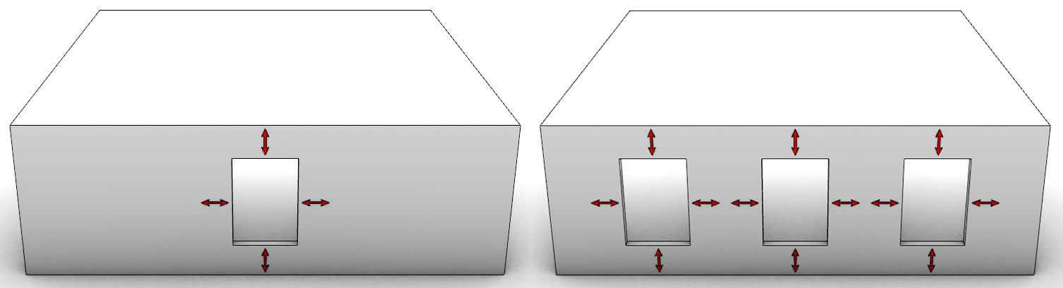
Fig. 1. Limited window shapes and locations on the wall.

Figure 2

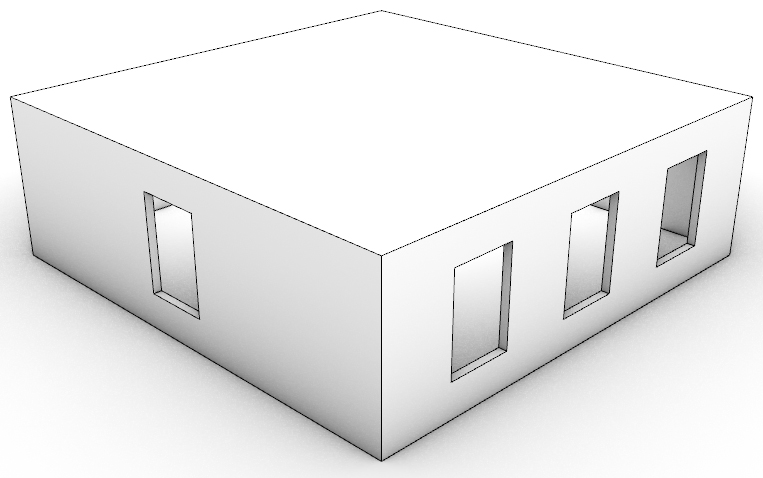
Fig. 2. Room with openings on two walls.

The fact that the previous models are not able to make predictions for these diverse openings heavily limits their adaptability, and these models do not provide a user-friendly experience to the architects who want to use this them to verify their designs, thereby undermining the practicality of such prediction models. The primary reason behind the restriction in existing research lies in the limitations of the tools used to create daylight simulation models. These tools can only generate simple variations within a narrow set of inputs. This study seeks to overcome these constraints and develop an improved model that can be applied to a wider range of scenarios.

2. Methodology

2.1. Research objective and workflow

The primary objective of this study is to design a neural network-based model capable of accurately predicting the annual daylight simulation results generated by the CBDM method for a target space. This neural network model is designed to effectively handle various challenging scenarios, including scenarios with single windows positioned off-center on the wall or multiple windows unevenly distributed on the wall, windows on the walls with varying dimensions, encompassing differences in heights, widths and sill heights, and situations where more than one wall contains windows, such as corner rooms and balconies.

The method development involves constructing a robust neural network-based model, and the entire workflow is visually represented in Fig. 3. The process consists of four essential parts: data generation, data processing, model training, and model validation. To achieve this, several tools and languages were employed, including (1) Rhino and Grasshopper, 3D-modeling platforms, (2) Honeybee-Radiance, a daylight simulation tool, (3) Python as the programming language, and (4) Scikit-Learn, a machine learning library that can implement a basic Artificial Neural Network (ANN) Model in Python.

Figure 3

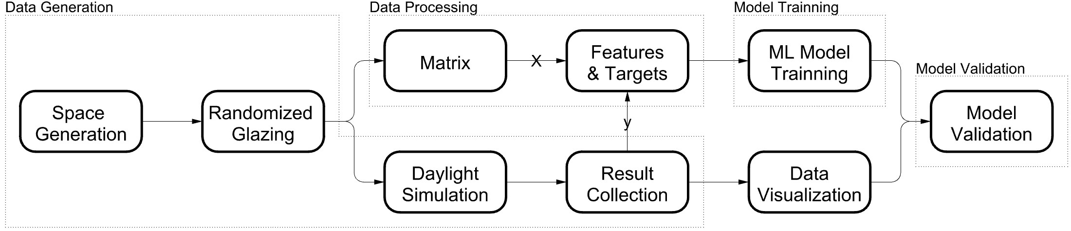
Fig. 3. Overall research workflow.

The core of this research lies in the data processing component, where the complex window shapes are converted into a series of matrices, which are then compiled into a set of features used for model training; this process is depicted in Fig. 4. Essentially, the method transforms the window information into a collection of 2D images, which are subsequently utilized as input features for training the neural network model.

Figure 4

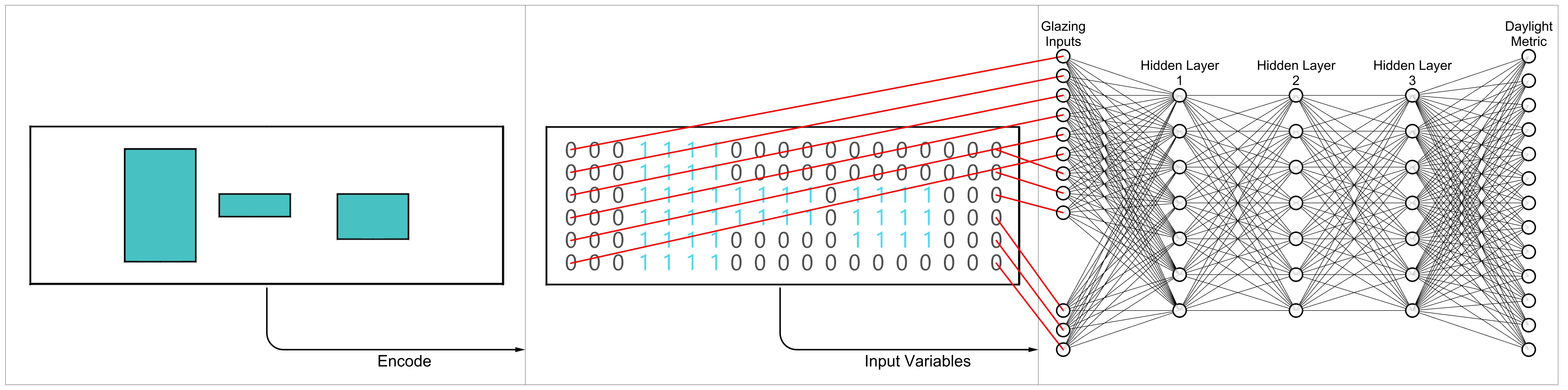
Fig. 4. Encoding openings into matrices for modeling training.

2.2. Encoding method

The matrix-based encoding approach illustrated in Fig. 4 offers significant advantages in enhancing the model’s adaptability to real-world scenarios. By encoding information about window openings on each wall into matrices, including the shapes of the windows and their relative positions, the model gains a more comprehensive understanding of the spatial arrangement.

The flexibility of this method is further highlighted by the matrix’s ability to expand with enough rows and columns. As long as the matrix has adequate dimensions, it can effectively handle any 2D shapes and varying numbers of windows, regardless of their complexity or arrangement. This adaptability makes the model well-suited for a diverse range of architectural designs, reflecting real-world conditions with varying window configurations.

Overall, this matrix-based encoding approach significantly enhances the model’s capability to predict daylight simulation results accurately for different building facades, providing practical and reliable insights for architects and designers in real-world applications.

2.3. Artificial neural networks

As mentioned earlier, the ANN model was employed in this study for daylight predictions. Artificial Neural Networks (ANNs) are computational models inspired by the structure and functionality of the human brain’s neural networks [9]. These networks consist of interconnected nodes, called artificial neurons or perceptrons, arranged in layers [9]. Information flows through these interconnected neurons, and each connection has an associated weight that modulates the signal [9]. ANNs are designed to learn from data, adapt to patterns, and make predictions or decisions based on the learned information [9]. The learning process involves adjusting the weights of the connections through various training algorithms, allowing the network to generalize and perform tasks beyond the training data [10]. ANNs have been applied in many different fields, such as computer vision, natural language processing, and finance, because of their capability to solve complex issues [11].

3. Research process

3.1. Data generation

3.1.1. Space generation

The ANN model heavily relies on having a sufficient amount of training data. To ensure coverage of all possible situations of window openings, a parametric model was developed using Rhino and Grasshopper. Rhino is a 3D modeling platform specifically used for space generation [12].

In this research project, a total of 5000 samples were generated. All the samples utilized a 30 by 30 by 10.5 ft box as the basis for simulating the testing space for daylight simulation, as illustrated in Table 1.

Table 1

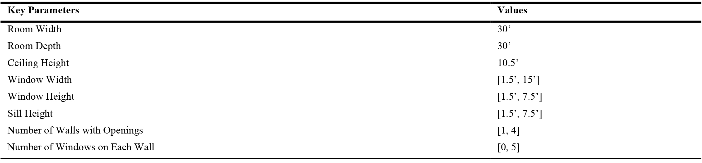
Table 1. Key parameters of the dataset.

3.1.2. Randomized openings

Grasshopper, a visual-based programming interface that operates within the Rhino environment [13], was utilized for this research. It enabled the creation of parametric models capable of generating an extensive range of variations by adjusting the inputs. Specifically, Grasshopper was employed to generate randomized window configurations on the walls of each of the 5000 samples, as depicted in Table 1. Each data sample in the dataset was designed to represent a 30 by 30 by 10.5 ft box, simulating the testing space for daylight simulation. For added versatility, the number of randomized openings on each wall varied from 0 to 5, covering a broad range of scenarios commonly encountered in office and home setups. Furthermore, key window parameters, such as window height, window width, sill height, and the number of windows on each wall, were also subjected to randomization for every data sample generated by Grasshopper. This extensive variation in the dataset enables the neural network model to better generalize and accurately predict daylight simulation results across diverse window configurations.

To make the randomized openings on each of the walls, as the Fig. 5 demonstrates, (1) the walls of the room were into 4 individual surfaces, where each of the surfaces has the same size, which is 30 ft by 10.5 ft, (2) an evenly spread, 19 by 6, point grid, which has 19 columns, index 0 to 18, and 6 rows, index 0 to 5 was generated on each of the surfaces, (3) a list of 10 non-repeating random integers was generated in Python, that range between 0 and 18, and then sorted in ascending order, for example, as shown in Fig. 5, the integers are: (1, 2, 4, 7, 8, 10, 11, 12, 15, 16), (4) the columns of points were kept based on the list of numbers that was generated in step 3, such as column 1, column 2, column 4, etc., and the remaining columns of points were discarded, (5) a set of random integers was generated in Python, that range between 0 and 5, in the case shown in Fig. 5 step 5, the integers are: (5, 4, 4, 3, 4, 1, 2, 2, 1, 5), (6) the list of numbers that was generated in step 5 was used to call out the points in the columns that were selected in step 4 accordingly, and (7) those 10 points were divided into 5 adjacent groups based on the column indices, where each group contained 2 points, and then rectangles were made based on those points.

Figure 5

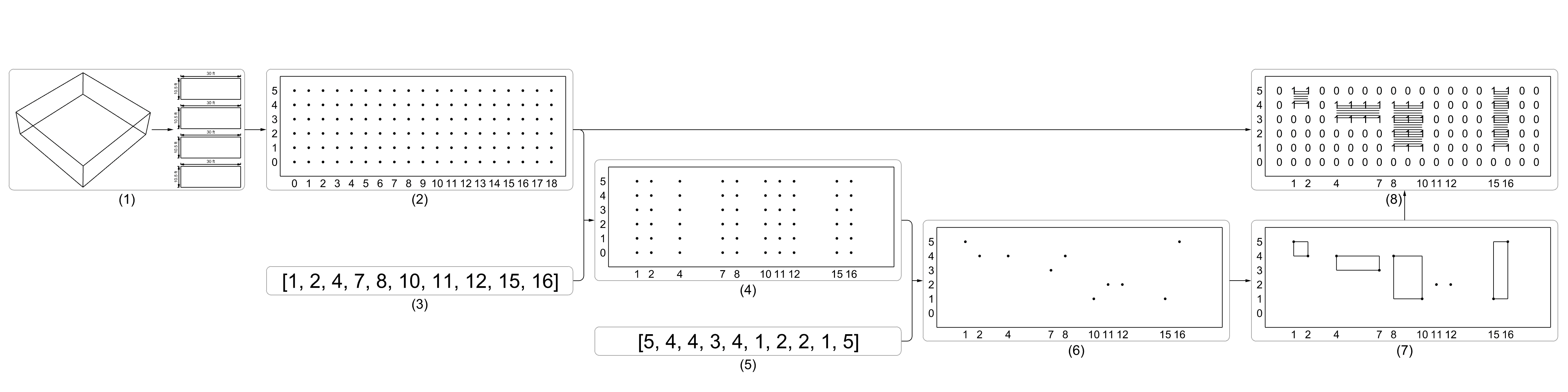
Fig. 5. Workflow of generating the randomized openings.

Since the algorithm that was used to determine the width of the randomized openings was set to generate 10 non-repeating random integers, theoretically, the single opening that has the maximum width will be generated when the random list made in step 3 is (0, 1, 2, 3, 4, 5, 6, 7, 8, 18) or (0, 10, 11, 12, 13, 14, 15, 16, 17, 18), which makes the maximum width of the window 15 ft. Meanwhile, maximum window height occurs when the random number group that was generated in step 7 has both 0 and 5 in it, which makes the maximum height of the window 7.5 ft. Therefore, the largest single opening possible that can be generated by this algorithm is 15 ft by 7.5 ft, which is 112.5 ft², while the wall is 315 ft², so the highest single window-to-wall ratio is 0.357. Notice that this is not the largest window-to-wall ratio possible that the algorithm can generate, when the 112.5 ft² opening appears, the other 4 windows can also achieve their maximum size, which is 1.5 ft by 7.5 ft, which makes it 11.25 ft², so in that case, the largest openings on one wall is 112.5 ft² + 11.25 ft² * 4 = 157.5 ft², which makes the window-to-wall ratio 0.5. And of course, by changing the density of the point grid and the default number of openings, this window-to-wall ratio can be increased dramatically.

Notice that in the example shown in Fig. 5, step 7, because one of the adjacent group of points has the same height, no rectangle was generated, so there are only 4 openings in this example. Therefore, based on the randomly selected points, the number of openings can vary from 0 to 5. Another thing to point out is that due to the limitations of this method, none of the openings can overlap with the others in the vertical direction.

3.1.3. Daylight simulation

Other than requiring detailed 3D models, which have been discussed in the previous paragraphs, performing CBDM simulations also requires detailed weather files as input, where each file corresponds to a specific location. For this project, Raleigh, North Carolina, was chosen as the location, and all the data files record the corresponding data from the Raleigh area. The weather data used for the simulations were from Ladybug’s epwmap database. Ladybug provides the capability to visualize and analyze weather data directly within Grasshopper; it offers a diverse range of visualization tools like sun path diagrams, wind roses, and psychrometric charts to better understand weather conditions at a particular location [14]. Additionally, Ladybug enables geometry studies, such as radiation analysis, shadow studies, and view analysis, which aid in optimizing building performance and energy efficiency based on weather patterns and solar positions, and all of these features are conveniently integrated into the Grasshopper environment [14]. Epwmap is a component developed as a part of Ladybug Tools, and its primary objective is to offer a unified interface for accessing all the freely available .epw weather files. By providing this centralized interface, epwmap simplifies the process of accessing and utilizing weather data from various sources within Ladybug Tools for climate analysis and simulations [15].

The simulation results generated by the CBDM methods were computed using Radiance, where Honeybee was used as the control mechanism within the Rhino-Grasshopper environment. Radiance is an engine developed by the Lawrence Berkeley National Laboratory in collaboration with the PG&E Pacific Energy Center [16]. It is used for energy-efficient lighting and daylighting strategies in building design, and it allows architects and designers to easily consider and implement energy-efficient lighting and daylighting strategies by providing access to libraries of materials, glazing, luminaires, and furniture [16]. Honeybee was developed as part of Ladybug Tools; in this project, Honeybee served as a Grasshopper plug-in designed to facilitate the creation, execution, and visualization of daylight simulations, and again, the computation core of Honeybee is Radiance [17].

Besides the 3D model and weather file, another important component for CBDM simulations is setting up the sensor grid. While sensor grid spacing does not heavily affect the accuracy of the CBDM simulation results [18], in order to reduce the amount of computation required, the spacing of the sensors was set up as 3 ft. Thus, for the 30 ft by 30 ft space, a 10 by 10 sensor grid was generated.

After all the preparations, the simulations were executed, and all the results were collected and embedded in CSV files. Examples can be seen in the data processing section.

3.1.4. Daylight metrics

Three daylight metrics were used in this research, including Daylight Autonomy (DA), Continuous Daylight Autonomy (cDA), and Useful Daylight Illuminance (UDI).

DA constitutes a daylight metric that determines sufficient daylight for productive occupancy without artificial lighting by considering work plane illuminance [19]. Designers and architects can refer to established guidelines in reference documents to ascertain the minimum illuminance levels required for different space types [19].

Proposed in 2006, cDA differs from earlier interpretations of daylight autonomy, cDA assigns fractional value to time intervals when daylight illuminance falls below the specified minimum level [19]. For instance, if a situation necessitates 800 lx and natural light provides 500 lx during a specific interval, a partial credit of 0.625 is accorded for that interval; consequently, instead of employing a strict threshold, this method introduces a more gradual transition between compliance and noncompliance [19].

UDI is a metric for evaluating indoor daylight quality. It replaces fixed threshold illuminance values with a range of illuminance levels considered beneficial [20]. Daylight levels below 100 lx are inadequate, 100–500 lx is effective, 500–2000 lx is desirable/tolerable, and above 2000 lx can cause discomfort; UDI considers illuminances within 100–2000 lx as useful, accommodating occupants’ visual needs [20]. This dynamic metric captures varying illuminance levels and preferences, offering a comprehensive assessment of indoor daylight quality; it’s applicable to diverse spaces and design variations, providing insight into occupants’ comfort and productivity [20]. In this research, daylight levels below 100 lx were marked as Useful Daylight Illuminance Low (UDI Low), and daylight levels above 2000 lx were marked as Useful Daylight Illuminance Up (UDI Up).

3.2. Data processing

3.2.1. Openings encoding

In this research, openings on the walls were encoded into matrices (Fig. 5, step 8). Data points within the openings and edges were set to 1, while the rest were set to 0. As Fig. 6 indicates, the four walls on the left were transformed into the matrices on the right, and the matrices were used as input variables for the ANN model. This matrix-based representation effectively captured information of the openings, enabling accurate predictions.

Figure 6

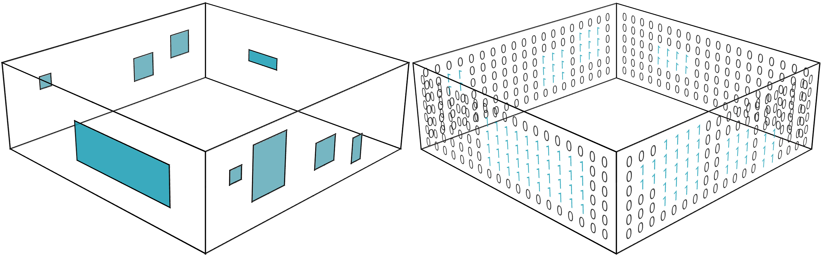
Fig. 6. Transforming information of the openings into matrices.

3.2.2. Features and targets

Figure 7 displays the input variables (X) for the ANN model, representing the openings on the walls. The dataset comprises 5000 rows and 456 columns. 5000 is the number of the data samples within the dataset. Each wall is depicted using a 19x6 point grid, resulting in 114 binary (0/1) data points per wall. As there are 4 walls, the total input features amount to 456.

Figure 7

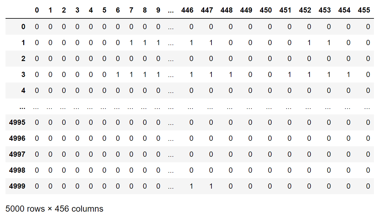
Fig. 7. Input variables (X) that mark the openings on 4 walls.

Figure 8 illustrates the target variables (Y) for the ANN model, representing the daylight autonomy (DA) results recorded by a 10x10 sensor grid. This dataset consists of 5000 rows and 100 columns, describing the targets for DA.

Figure 8

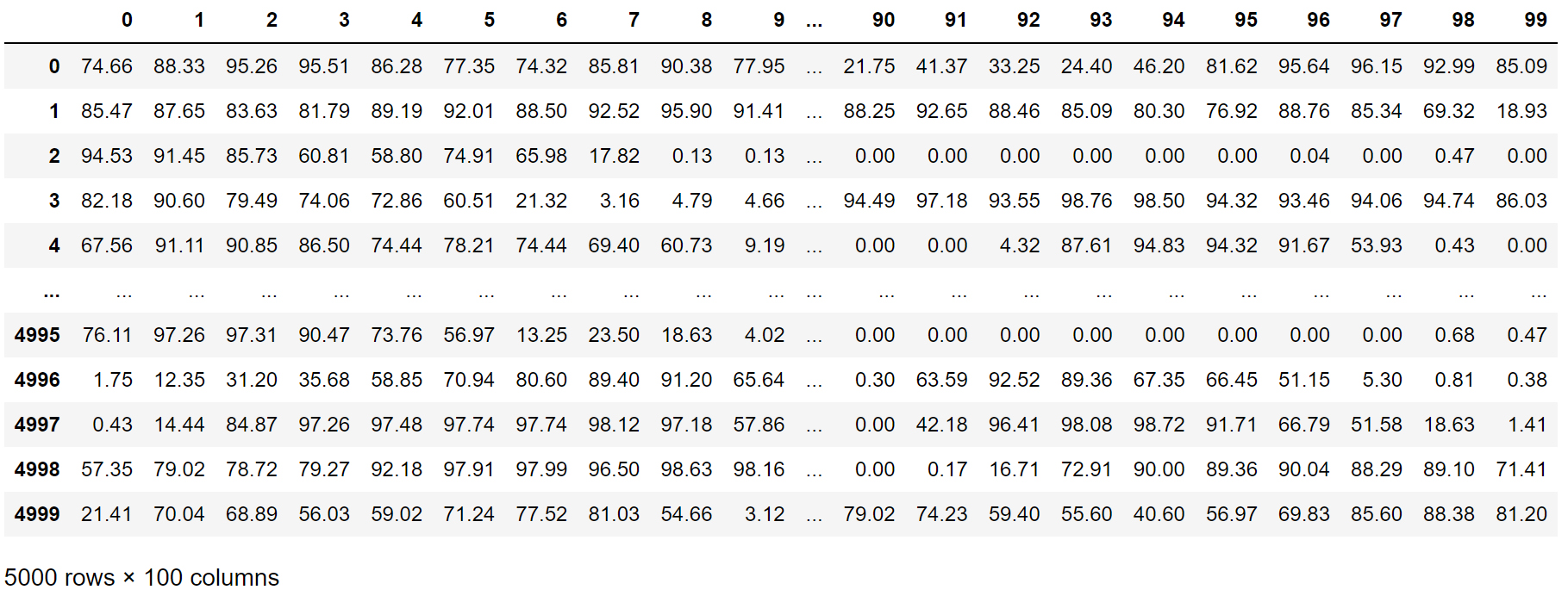
Fig. 8. Target variables (Y) that mark the DA simulation result of the 10 by 10 sensor grid.

It is worth noting that this research compared the ANN model’s performance across different metrics, including DA, cDA, and UDI. Although Fig. 8 demonstrates only the simulation result for DA, the other daylight metrics’ simulation results were also included in the same data structure.

3.3. Model training

3.3.1. ANN architecture and parameters tuning

The process of training and testing the ANN model is iterative. It involves tuning the hyperparameters and optimizing the model architecture to achieve better performance on the test set while avoiding overfitting on the training data. In this tuning process, the goals are to tune the model so that it can generalize well to new data and make accurate predictions on different daylight metrics, and to find a reasonable size of the training set for the ANN model while maintaining a high accuracy.

Training the ANN model for this research took 8 steps. The first step is data preprocessing, where the data was prepared, which has been presented in the previous section; in some of the cases, no window was generated on any of the 4 walls, and those cases were removed. The second step is splitting the data, where the dataset was divided into a training set and a test set. The training set was used to train the ANN model, while the test set was used to evaluate the ANN model’s performance on unseen data; in this project, the train/test ratio was set as 10 to 1. As the size of the training set varies, the size of the testing set changes accordingly. The third step is model initialization; in this step, the ANN model from scikit-learn [21] was chosen to be trained, and to make the predictions. The fourth step is model compilation, where the default optimizer from scikit-learn was used to determined how the model is updated based on the calculated gradients; the square error was chosen as the loss function and the R-squared value was used as evaluation metric which provides a performance measure during training. The fifth step was mode training, where the training data, which can be seen in Figs. 7 and 8, was fed into the ANN model; the data helps the model learn the relationships between the input variables (X) and the target variables (Y). The sixth step is performance evaluation; after training, the model was evaluated using the test set to assess its accuracy and generalization capability on unseen data. The seventh step is hyperparameter tuning, where the hyperparameters of the model were adjusted to improve the model’s performance; as Fig. 9 demonstrates, the learning rate was set to 0.005, the number of layers was set to 3, and the number of neurons was set to 300 for each layer. The eighth and final step is prediction on unseen data; after the ANN model was trained and tuned, it was used to make predictions on completely new and unseen data, which can be seen in the following section.

Figure 9

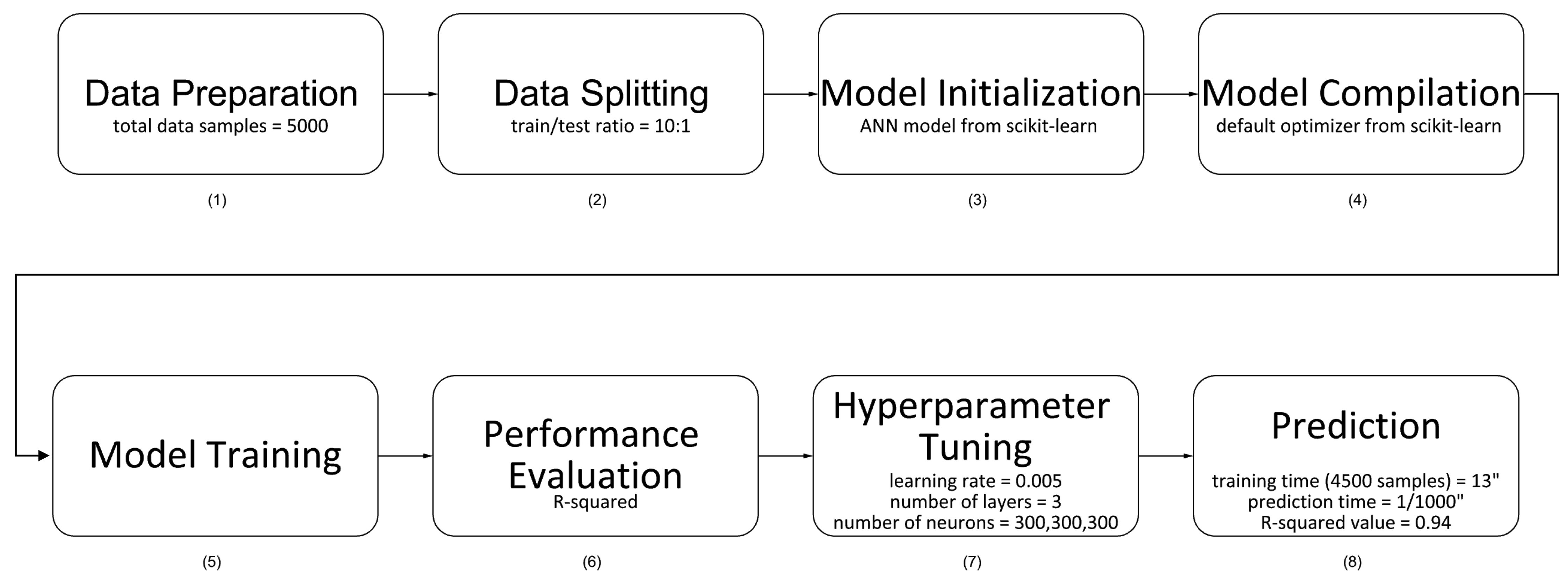
Fig. 9. Process of training the ANN model.

4. Results

4.1. Accuracy and efficiency

To evaluate and compare the performance of the ANN model across distinct daylight metrics and varying dataset sizes, Fig. 10 was generated to visually represent the outcomes. The ANN model was applied to predict diverse categories of daylight metrics, encompassing DA, cDA, and UDI. Figure 10 distinctly illustrates that both DA and cDA exhibit high accuracy levels, with cDA displaying particularly high performance; when the dataset size approximates 1700 samples, the cDA predictions achieve a notably high R-squared value of 0.95, highlighting the model’s exceptional predictive abilities. Although the R-squared value for UDI is not as high, the model still manages to reach an R-squared value of 0.9 when the dataset size is around 4000 samples.

Figure 10

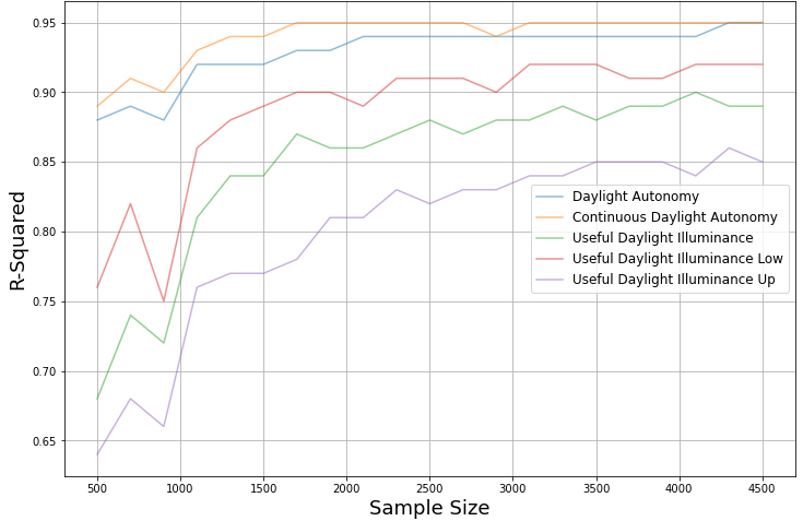
Fig. 10. ANN prediction accuracy among different daylight metrics.

However, the ANN model’s performance varies among different ranges of illuminance; as shown in Fig. 10, when predicting Useful Daylight Illuminance Low, where the sensors get lower than 100 lx illuminance, the R-squared value of the prediction accuracy reaches 0.9 with only 1700 samples; on the other hand, when making predictions of Useful Daylight Illuminance Up, where the sensors get higher than 2000 lx illuminance, the R-squared value of the prediction accuracy just reaches 0.77 when the number of the samples is 1700. In order to increase the R-squared value to 0.9, 3500 cases are needed, which is more than doubled the number of samples needed to achieve such accuracy in the Useful Daylight Illuminance Low prediction.

As depicted in Fig. 11, in order to demonstrate the model’s precision visually, an external sample was introduced to the ANN model. On the left, the DA result was generated by the CBDM method, whereas the DA result on the right was predicted by the ANN model. While noticeable discrepancies between the CBDM-generated data and the ANN model’s predictions exist for specific data points, the overall trends remain the same. Evidently, the ANN model has effectively captured the correlations between window configurations, their relative positions on walls, and ensuing DA outcomes.

Figure 11

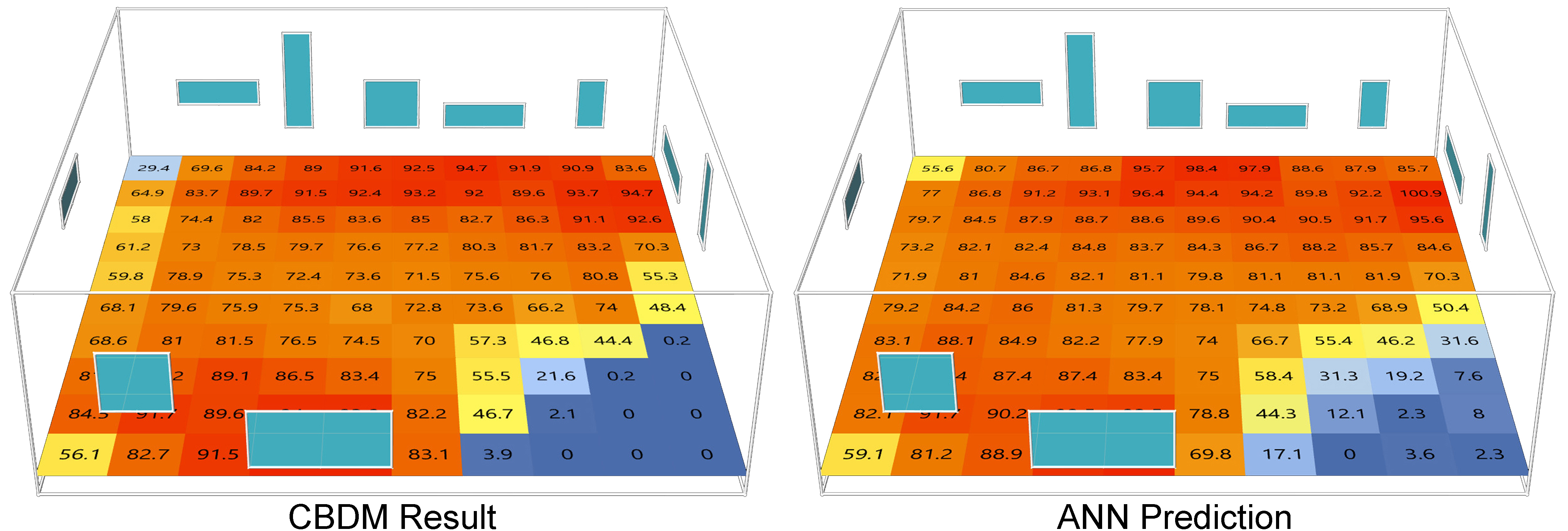
Fig. 11. CBDM result vs ANN model prediction.

In the computer that was used to perform this research, which is equipped with an Intel i7-9700 CPU, it takes Honeybee and Radiance more than 15 seconds on average to run a simulation with one result. This difference is striking when comparing this to the performance speed for the ANN model. As Fig. 9 indicates, with the same hardware, the ANN model can train the model using 4500 samples in less than 13 seconds. In addition, making the prediction depicted in Fig. 11 takes even less time, under 1/1000 seconds. This speed is impressive, especially considering that the accuracy remains high.

5. Discussion

As the results show, the method introduced in this research shows great accuracy and efficiency when making predictions for annual daylight simulation results over different types of daylight metrics. With only 2000 samples, the R-squared value of the prediction accuracy reached 0.95 in Continuous Daylight Autonomy, 0.93 in Daylight Autonomy, and 0.86 in Useful Daylight Autonomy. It is worth noting that many of the samples in the test set have windows on more than one wall; meanwhile, all those windows that populate the walls have variations over height, width, sill height, and their relative locations on the walls, which none of the previous machine learning-based models are capable of making daylight predictions for. Furthermore, the ANN model demonstrates great efficiency in making predictions; with the same hardware that was used for conducting this research, performing one CBDM simulation with Honeybee and Radiance takes more than 15 seconds on average; however, it only takes the ANN model 13 seconds to train 4500 samples, where making each prediction takes less than 1/1000 seconds.

However, when considering making predictions over different ranges of Useful Daylight Illuminance, the prediction accuracy over the high range, which is higher than 2000 lx, was not as robust as the prediction accuracy over the low range, which is lower than 100 lx. The reason behind this performance difference may be related to the feature of the samples within the dataset. Although most of the rooms within the dataset had at least one window and many of them have multiple, as mentioned, the highest single window-to-wall ratio is 0.357, so the likelihood that the sensors record an illuminance higher than 2000 lx is very low; therefore, the ANN model didn’t get enough training data to understand the relationship between the window configurations and the distribution of Useful Daylight Illuminance above 2000 lx, which resulted in its poor performance when making predictions over the high range. To the contrary, many of the samples within the dataset had a low window-to-wall ratio, which contributed to a lower amount of daylight penetrating into the space; this resulted in many of those sensors within the sensor grid recording an illuminance lower than 100 lx, which falls into the lower range of the Useful Daylight Illuminance, so these data points were more common in the dataset, and therefore the ANN model was able to better make these predictions. Therefore, to guarantee better performance of the ANN model when making predictions over Useful Daylight Illuminance Up, more samples with higher window-to-wall ratios can be employed in the future datasets.

The introduction of machine learning, deep learning, and other artificial intelligence-based models into the field of daylight simulation has been a popular research topic; however, utilizing matrices derived from geometric data to train ANN models is a significant leap forward in addressing the challenge of daylight simulation brought by the variations of window configurations. One notable strength of this methodology lies in its adaptability; the method proposed in this research study can be applied to other fields of building science, such as energy consumption simulation and thermal comfort prediction.

Even though many promising artificial intelligence applications have emerged, perceiving, analyzing, and generating 3D-spaces remains challenging; by encoding 3D information into 2D matrices, this study shows that the ANN model has the ability to gain comprehensive understanding of spatial arrangements, and demonstrates its ability to make accurate predictions over annual daylight simulation results. The dimension-reducing method that was introduced in this research has the potential to be applied in other artificial intelligence methods, which can help future models gain better understanding of the 3D environment and make great applications.

6. Conclusion

This study introduces an innovative approach utilizing ANN models to predict CBDM simulation outcomes, incorporating more versatile window configurations. The effectiveness and dependability of this approach are evident in the ANN model’s prediction accuracy across various daylight metrics. Geometric data was translated into matrices, which can be described as a dimension-reducing process that transforms 3D geometrical details into matrices, such matrices can be considered as a collection of binary 2D images. The ANN effectively grasps the correlation between these matrix-based inputs and the CBDM simulation outcomes. For instance, with only 1700 samples, the R-squared value of the prediction accuracy can reach 0.95 in Continuous Daylight Autonomy, while maintaining extremely high efficiency in comparison with the traditional CBDM process. Nonetheless, the current ANN-based model exhibits limitations when extending to other factors of the building environment, such as location, orientation, ceiling height, shading devices, room dimensions, wall thickness, etc. While some of these constraints could potentially be mitigated by expanding the dataset size, others, such as ceiling height and room dimensions, require more intricate solutions, possibly involving certain forms of Deep Learning techniques.

Encouragingly, the matrix-based input methodology holds considerable promise, not only for the ANN model but also for diverse machine learning, deep learning, and other Artificial Intelligence methods. Concurrently, this methodology holds potential for predicting energy consumption, thermal comfort, and other aspects pertinent to research within building science.

Acknowledgment

This research was funded by North Carolina State University’s summer research fellowship.

Contributions

Conceptualization, D.W. and W.P.; methodology, D.W., J.H. and S.C.; software, D.W.; validation, D.W., W.P. and J.H.; resources, W.P.; data curation, D.W.; writing—original draft preparation, D.W.; writing—review and editing, J.H., W.P., S.C. and T.Y.; visualization, D.W., X.Z. and Z.T.; supervision, W.P. and J.H.; project administration, W.P.; funding acquisition, W.P.

Declaration of competing interest

The authors declare no conflict of interest.

Data availability statement

All the data that has been used within this research was created by the corresponding author, and all the datasets and the python file can be found at: https://drive.google.com/drive/folders/11QqBIkkJQXMlCYo7EJ0bZoUuN4sEMpB0?usp=drive_link

References

N.E. Klepeis, W.C. Nelson, W.R. Ott, J.P. Robinson, A.M. Tsang, P. Switzer, J.V. Behar, S.C. Hern, and W.H. Engelmann, The National Human Activity Pattern Survey (NHAPS): A Resource for Assessing Exposure to Environmental Pollutants, Journal of Exposure Science & Environmental Epidemiology 11 (2001) 231-252. https://doi.org/10.1038/sj.jea.7500165
F. Beute, Powered by Nature: The Psychological Benefits of Natural Views and Daylight, Technische Universiteit Eindhoven, Eindhoven, 2014.
M. Ayoub, 100 Years of Daylighting: A Chronological Review of Daylight Prediction and Calculation Methods, Solar Energy 194 (2019) 360-390. https://doi.org/10.1016/j.solener.2019.10.072
P. Moon and D.E. Spencer, Illumination from a Non-uniform Sky, Illumination Engineering 37 (1942) 707-726.
P.R. Tregenza and I.M. Waters, Daylight Coefficients, Lighting Research & Technology 15(2) (1983) 65-71. https://doi.org/10.1177/096032718301500201
J. Mardaljevic, Examples of Climate-Based Daylight Modelling, in: CIBSE National Conference, 2006, pp. 1-11, UK.
M. Ayoub, A Review on Machine Learning Algorithms to Predict Daylighting Inside Buildings, Solar Energy 202 (2020) 249-275. https://doi.org/10.1016/j.solener.2020.03.104
H. Nourkojouri, N.S. Shafavi, M. Tahsildoost, and Z.S. Zomorodian, Development of a Machine-Learning Framework for Overall Daylight and Visual Comfort Assessment in Early Design Stages, Journal of Daylighting 8 (2021) 270-283. https://doi.org/10.15627/jd.2021.21
S. Haykin, Neural Networks: A Comprehensive Foundation, Prentice Hall, New Jersey, 1998.
I. Goodfellow, Y. Bengio, and A. Courville, Deep Learning, MIT Press, Massachusetts, 2016.
Y. LeCun, Y. Bengio, and G. Hinton, Deep Learning, Nature 521 (2015) 436-444. https://doi.org/10.1038/nature14539
Rhino Overview, 2023. Available at: https://www.rhino3d.com/features/ (Accessed: 20 July 2023). https://doi.org/10.1177/0748730409335546
Grasshopper, 2023. Available at: https://www.rhino3d.com/features/#grasshopper (Accessed: 20 July 2023).
Ladybug Tools, 2023. Available at: https://www.food4rhino.com/en/app/ladybug-tools (Accessed: 20 July 2023).
Epwmap, 2023. Available at: https://github.com/ladybug-tools/epwmap (Accessed: 20 July 2023).
Desktop Radiance, 2019. Available at: https://www.radiance-online.org/archived/radsite/radiance/desktop.html (Accessed: 20 July 2023).
Honeybee, 2022. Available at: https://www.ladybug.tools/honeybee.html (Accessed: 20 July 2023).
E. Brembilla and J. Mardaljevic, Climate-Based Daylight Modelling for Compliance Verification: Benchmarking Multiple State-of-the-art Methods, Building and Environment 158 (2019) 151-164. https://doi.org/10.1016/j.buildenv.2019.04.051
C.F. Reinhart, J. Mardaljevic, and Z. Rogers, Dynamic Daylight Performance Metrics for Sustainable Building Design, Leukos 3 (2006) 7-31. https://doi.org/10.1582/LEUKOS.2006.03.01.001
A. Nabil and J. Mardaljevic, Useful Daylight Illuminances: A Replacement for Daylight Factors, Energy and Buildings 38 (2006) 905-913. https://doi.org/10.1016/j.enbuild.2006.03.013
Neural Network Models, 2023. Available at: https://scikit-learn.org/stable/modules/neural_networks_supervised.html#regression (Accessed: 20 July 2023).

Get PDF (7.48 MB)

SHARE ON