Volume 12 Issue 2 pp. 278-292 • doi: 10.15627/jd.2025.19
Determination of Efficiency of the Vertical Specularly Reflecting Cylindrical Light Shaft for Different Types of Firmaments
Serhii Litnitskyi,* Eugene Pugachov, Taras Kundrat, Vasyl Zdanevych
Author affiliations
Department of Architectural Design Fundamentals, Construction and Graphics, Institute of Civil Engineering and Architecture, National University of Water and Environmental Engineering, Rivne, Ukraine
*Corresponding author.
gavran88@ukr.net (S. Litnitskyi)
pev1957@ukr.net (E. Pugachov)
kundratt@i.ua (T. Kundrat)
vasyl.zdanevych@gmail.com (V. Zdanevych)
History: Received 13 February 2025 | Revised 1 May 2025 | Accepted 17 May 2025 | Published online 20 July 2025
2383-8701/© 2025 The Author(s). Published by solarlits.com. This is an open access article distributed under the terms and conditions of the Creative Commons Attribution 4.0 License.
Citation: Serhii Litnitskyi, Eugene Pugachov, Taras Kundrat, Vasyl Zdanevych, Determination of Efficiency of the Vertical Specularly Reflecting Cylindrical Light Shaft for Different Types of Firmaments, Journal of Daylighting, 12:2 (2025) 278-292. doi: 10.15627/jd.2025.19
Figures and tables
Abstract
Article is devoted to determination of efficiency of the vertical specularly reflecting cylindrical light shaft for various types of the firmaments standardized by CIE (International Commission on Illumination). Efficiency of the light shaft was calculated as the relation of the output luminous flux (exiting through the lower base of the shaft) to the entering luminous flux (entering through the upper base of the shaft). The output luminous flux consists of the luminous flux created by direct light (gets on base of the shaft directly from the sky) and the luminous flux created by light which is repeatedly reflected from its inner side surface. For the 4th and 15th types of firmaments surfaces of dependence of the total efficiency (formed by the direct and reflected light) of the light shaft from solar time and the index of the shaft and also – graphs of dependence of total efficiency of the light shaft on the index of the shaft are given. For the 4th types of firmament the maximum values correspond to solar noon (from 29.3% to 96.3%), and the minimum values are at sunrise and sunset (from 28.7% to 95.3%). For the 15th types of firmament the maximum values correspond to solar noon (from 15.5% to 95.8%), and the minimum values are at sunrise and sunset (from 13% to 91.5%). The results showed that the solar time has almost no effect on the efficiency of the light shaft, which allows us to average the results in a certain way. As the light shaft index increases, that is, as the ratio of the radius to the shaft height increases, the efficiency value asymptotically approaches one hundred percent, which is physically correct. Knowing the radius, height, index of the shaft and the specular reflection coefficient of its inner surface, it is possible to predict natural lighting under the shaft and use energy resources more rationally.
Keywords
light shaft, natural illumination, firmament, repeated luminous reflectance
Nomenclature
| \(\mathrm{\Omega}\) | the solid angle limiting the luminous flux falling on the plane, sr |
| \(dE_H\) | the illumination of the plane perpendicular to the axis of the elementary solid angle d\(\mathrm{\Omega}\), created by the elementary radiator within this solid angle, klx |
| \(cos{\beta_x},cos{\beta_y},cos{\beta_z}\) | radiation importance functions for the illumination of coordinate planes |
| \(\beta_x, \beta_y, \beta_z\) | light inclination angles on coordinate planes yOz,xOz,xOy, rad |
| \(dS\) | area of the elementary plane of the firmament |
| l | distance from the middle of the elementary plane dS to the calculation point, m |
| \(\varepsilon_z\) | z-coordinate of the light vector, lm |
| \(t_z\) | z-coordinate of the unit vector |
| \(\buildrel t\over t\rightarrow\) | the unit vector |
| \(\theta\) | the angle between the unit vector and the vector of the normal to the radiator surface, rad |
| S | integration area |
| \(L_\theta\) | brightness of any element of the firmament, cd/m2 |
| \(L_Z\) | brightness in the zenith, cd/m2 |
| \(\phi(Z)\) | luminance gradation function |
| \(f(\chi)\) | scattering indicatrix function |
| \(\gamma_S\) | angular height of the Sun, rad |
| \(E_V\) | horizontal extraterrestrial illuminance, klx |
| \(D_V\) | diffusion horizontal illumination, klx |
| \(T_V\) | luminous turbidity factor |
| \(K_P\) | efficiency of the light shaft, % |
| \(F_{in}\) | entrance luminous flux, klx |
| \(F_{out}^{str}\) | part of the output luminous flux created by direct light from the firmament, klx |
| \(F_{out}^{ref}\) | part of output luminous flux created by light which is repeatedly reflected from side face of the light shaft, klx |
| R | radius of the cylindrical light shaft, m |
| RP | reference point |
| \(\varepsilon_z\) | z-coordinate of the light vector, which is created by the elementary plane at the reference point, lm |
| \(\varepsilon_z^B\) | z-coordinate of the light vector at the reference point, created by direct light that passed through the upper base of the shaft, lm |
| H | shaft height, m |
| N | number of reflections of the beam from walls of the light shaft |
| z | z-coordinate of the center of the reflecting plane dS, m |
| \(\rho\) | specular reflection coefficient of its inner surface |
| \(L_{in}\) | beam brightness at the entrance to the light shaft, cd/m2 |
| \(L_{out}\) | output beam brightness from the light shaft, cd/m2 |
| \({\vec{\varepsilon}}^{out}\) | light vector created in the reference point on the basis of the light shaft by light reflected from the plane, lm |
| \(\varepsilon_z^{out}\) | z-coordinate of the light vector created in reference point reflected from all inside face of the shaft, lm |
| \(\psi\) | declination of the Sun, rad |
| \(\omega\) | time angle, rad |
| \(\varphi\) | latitude, rad |
| \(\alpha_S\) | azimuth of the Sun, rad |
| Nd | day number of the year |
| \(t_S\) | solar time, h |
| \(t_{\mathrm{sunrise}}\) | solar sunrise time, h |
| \(t_{\mathrm{sunset}}\) | solar sunset time, h |
| M | the total number of generated points during integration by the Monte-Carlo method |
| \(\delta\) | relative accuracy |
1. Introduction
Natural lighting plays very important role in human life. Its insufficient quantity or absence not only affects destructive image human health, but also causes different inconveniences almost in all fields of activity of mankind. However and the surplus of lighting has negative effect. Therefore, more and more adequate mathematical distribution models of brightness on firmament are being developed, which are the source information for modeling natural lighting both outside and inside buildings through light openings of various shapes and locations, for example, through light shafts.
In particular, till 2004 for calculation of brightness of the sky and natural illumination and other characteristics of the light field used the document CIE S 003/E:1996 (ISO 15469:1997) "CIE standard overcast sky and clear sky" [1] which mathematically described distribution of brightness on firmament with continuous overcast the formula Moon-Spencer offered by the American scientists Moon and Spencer in 1942.
Later the International commission on illumination has standardized the new document: CIE S 011/E:2003 (ISO 15469: 2004(E) Spatial distribution of daylight – CIE standard general sky) [2]. A similar document, namely DSTU ISO 15469:2008. “Spatial distribution of daylight brightness. Standard cloudy and cloudless sky according to CIE (ISO 15469:2004, IDT)” [3] – was introduced in Ukraine. 15 mathematical models of types of firmaments are already given in both standards, and the firmament with continuous overcast is only one of them (the first). The mentioned documents are still rather new and therefore demand both the additional analysis and correct application (adaptation), in particular, for conditions of Ukraine.
Since on the firmament is different for all models, the natural lighting they create will also be different. Information on the number of natural illumination which it is possible to expect in this area (light resources) allows to project more rationally light openings in buildings and constructions for reduction of use of artificial lighting, losses of heat energy in the winter and energy costs of conditioning.
Various aspects of the above-mentioned mathematical models of types of firmaments have been studied in works [4-10]. In works [11-12], the types of sky firmaments characteristic of Ukraine in different months of the year were determined. Similar problems were solved for Singapore [13], Chile [14] and Hong Kong [15]. In work [16], an analysis was conducted to determine the ratio of the brightness of an arbitrary element of the sky to the brightness at the zenith.
One of the factors characterizing natural lighting resources is the diurnal course of illumination of the horizontal plane created by different types of firmaments on typical days of the year at a given latitude. For the first type of firmament (standard overcast sky according to CIE), the illumination of the horizontal plane does not change during the day, since the brightness distribution over the sky (Moon-Spencer formula) does not depend on the position of the Sun and, accordingly, solar time. For the remaining 14 types of firmaments, the coordinates of the Sun must be taken into account when calculating, since the distribution of brightness across the sky depends on them and affects the illumination of the horizontal plane and, in general, the illumination of any plane or surface.
The course of illumination of the horizontal plane, in particular, allows you to determine critical outdoor lighting, which is associated with the duration of use of artificial lighting in a given area.
Modeling horizontal illumination from different types of skylights also allows you to design illumination in buildings for various purposes with light openings of a certain shape, for example, in the form of light shafts. To estimate the illumination under a light shaft, it is important to know the efficiency of the light shaft and how much it depends on the type of firmament (brightness distribution across the sky).
A light shaft is a light opening, most often vertical, of any cross-section [17-22]. It differs from a skylight in that a significant portion of the light shaft's output light flux is light repeatedly reflected from its inner walls. And it differs from a light pipe in that in a light pipe the output light flux creates only multiple reflected light, and direct light does not fall on the area of the output opening [23-31].
Light shafts were widely used in industrial, public and partially in residential buildings [32-33]. Upper lighting through light shafts is projected in buildings (rooms) which on their functional purpose and the space decision have the low ceiling and big coating thickness, when there is no side lighting or the depth of the room does not allow to provide regulatory requirements on natural lighting by means of side lighting. Light shafts also quite often use as the design solution of the interior. Figure 1 shows some examples of light shaft shapes encountered in architectural and construction practice. Light shafts of simple forms are most often applied: cylindrical vertical or inclined, in the form of the parallelepiped, the cut-off cone, the cut-off pyramid. This is, in particular, due to the complexity of modeling illumination from light shafts, especially modeling illumination created by multiple reflections of light inside the shaft. The side surface of shafts with specular reflection is usually made glossy in light colors. In an ideal situation, there is no roughness or defects on the side surface. Therefore, it can be assumed that the sun's rays inside the shaft are reflected according to the law of geometric optics (specularly). In architectural and construction practice, shafts with diffuse light reflection are also used when it is necessary to create soft, diffused light. However, they are inferior to specular shafts in terms of efficiency.
Figure 1
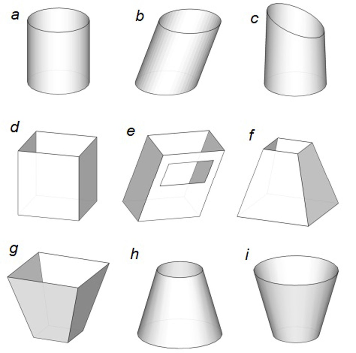
Fig. 1. Examples of forms of light shafts which often meet in architectural and construction practice: (a) vertical cylindrical shaft; (b) inclined cylindrical shaft; (c) cylindrical shaft with non-horizontal upper base; (d) parallelepiped shaft; (e) a shaft in the form of an inclined parallelepiped with a rectangular opening; (f) truncated pyramid shaft; (g) a shaft in the form of a truncated pyramid with the top down; (h) a shaft in the form of a truncated circular cone; (i) a shaft in the form of a truncated circular cone with the top down.
The article aims to analyze whether the efficiency of a vertical specularly reflecting cylindrical light shaft will change during a sunny day at a latitude of 50° N for different types of firmaments.
The methods and materials section describes how the natural lighting of a plane according to [2] and [34] and the efficiency of a cylindrical light shaft are calculated in general terms. To calculate the efficiency, it is necessary to know the input and output luminous fluxes. Moreover, the output light flux consists of the light flux created by direct light and the light flux created by light repeatedly reflected from the side surface of the light shaft. The calculations and results section provides the input datas for calculating the efficiency and demonstrates the results obtained for the 4th type of firmament (overcast, moderately graded and slight brightening towards the Sun) and the 15th type of firmament (white-blue turbid sky with broad solar corona). The discussion section provides an analysis of the results obtained and directions for possible further research. The conclusions briefly describe the obtained results.
2. Methods and materials
In the general view the illumination of the plane is determined by the formula [35]:
where \(\Omega\) – the solid angle limiting the luminous flux falling on the plane, sr; \(dE_H\) – the illumination of the plane perpendicular to the axis of the elementary solid angle \(d{\Omega}\), created by the elementary radiator within this solid angle, klx; \(cos{\beta_x}\), \(cos{\beta_y}\), \(cos{\beta_z}\) – radiation importance functions for the illumination of coordinate planes (\(\beta_x\), \(\beta_y\), \(\beta_z\) – light inclination angles on coordinate planes \(yOz\),\(xOz\),\(xOy\)).
Illumination of the horizontal plane can be calculated as the module of the sum of z-coordinates of the light vectors created by elementary plane dS of the firmament. In view of the fact that \(d\Omega=\frac{cos{\theta}}{l^2}dS\), the formula for calculating of z-coordinate of the light vector can be written as
where \(t_z\)– z-coordinate of the unit vector \(\buildrel t\over t\rightarrow\), sent from the middle of the elementary plane dS to the reference point; l – distance from the middle of the elementary plane dS to the calculation point, m; \(\theta\) – the angle between the vector \(\buildrel t\over t\rightarrow\) and the vector of the normal to the surface of the radiator, rad; S– integration area; \(L_\theta\)– brightness of any element of the firmament which is calculated on the formula [2]:
where \(\phi\) – function of gradation of brightness which connects the firmament element brightness (elementary plane) and its zenith angle; f – the dispersion indicatrix connecting the relative brightness of element of firmament with its angular distance from the Sun; \(L_Z\) – firmament brightness in zenith. Functions φ and f are also defined according to the formulas given in ISO 15469: 2004. For the first six mathematical models of types of firmaments brightness in the zenith L_Z is calculated on the formula [34]:
and for other models it is calculated by the formula [34]:
where \(\gamma_S\) – angular height of the Sun, rad; \(E_V\) – horizontal extraterrestrial illuminance, klx; \(D_V\) – diffusion horizontal illumination, klx; \(T_V\) – luminous turbidity factor; A,B,C,D,E – the parameters specified in [34].
2.1. Calculation of efficiency of the light shaft
The efficiency of the light shaft is determined by the formula:
where \(F_{in}\) – entrance luminous flux, klx; \(F_{out}^{str}\) – part of the output luminous flux created by direct light from the firmament, klx; \(F_{out}^{ref}\) – part of output luminous flux created by light which is repeatedly reflected from side face of the light shaft, klx.
It should be noted that some of the output light is always lost, so \(F_{out}^{str}+F_{out}^{ref}\) less than \(F_{in}\), and \(K_P\) less than 100%.
2.2. Calculation of the entrance luminous flux
The entrance luminous flux can be defined as the product of the module of z-coordinate of light vector (illumination of the upper basis of the shaft) calculated by formula (2) on the area of the upper basis. As the upper basis has the circle form, the entrance flux is equal:
where R – radius of the cylindrical light shaft, m.
2.3. Calculation of the output luminous flux created by direct light
The part of the firmament lighting the reference point RP on the lower base of the shaft is formed at the intersection of the celestial hemisphere of unit radius (centered at the calculated point) with a conical surface, the vertex of which is the calculated point, and the directrix is the circle of the upper base of the shaft (Fig. 2). Then the illumination in the reference point created by direct light from the firmament can be determined on the known formulas by integration within the solid angle formed by the cone, using upper base of the shaft (cone), but not mentioned area on the celestial sphere of unit radius as it is more difficult to define its borders (the cone and area on the celestial hemisphere limit the identical solid angle).
Figure 2
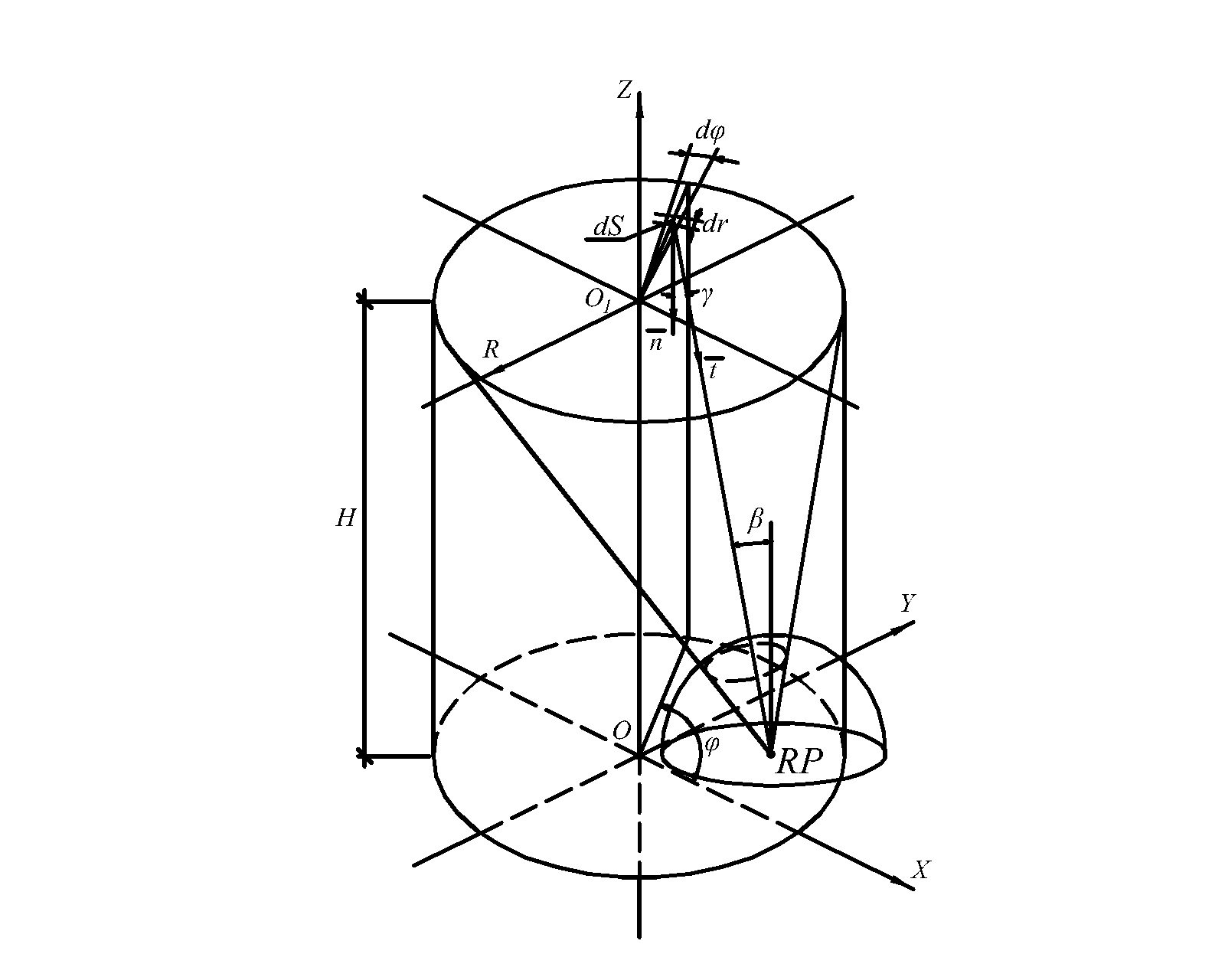
Fig. 2. To determination of illumination by direct light of the reference point RР of the lower base of the light shaft.
Z-coordinate of the light vector, which is created by the elementary plane \(dS=rd\phi dr\) at the reference point, is determined by the formula [36]:
and z-coordinate of the light vector at the reference point, created by direct light that passed through the upper base of the shaft, is calculated by integrating [36]:
The module of z-coordinate of light vector on the lower horizontal base of the shaft is equal in the reference point to its illumination.
To calculate the output light flux, a radial grid is divided on the lower base of the shaft (29 points along the radius and 34 points along the external circle, Fig. 3), at the nodes of which the illumination is determined. Then the average illumination value for each cell was calculated (for triangular cells - the average of three, and for quadrilateral - of four values). The necessary minimum quantity of nodes was defined as a result of computer experiments, that further increase in quantity of nodes of the grid did not affect significantly result of calculations. The output luminous flux \(F_{out}^{str}\) created by direct light was calculated as the sum of the flows passing through all cells of the grid. And the flux passing through one cell was calculated as the product of the average illumination of the cell and its area.
Figure 3
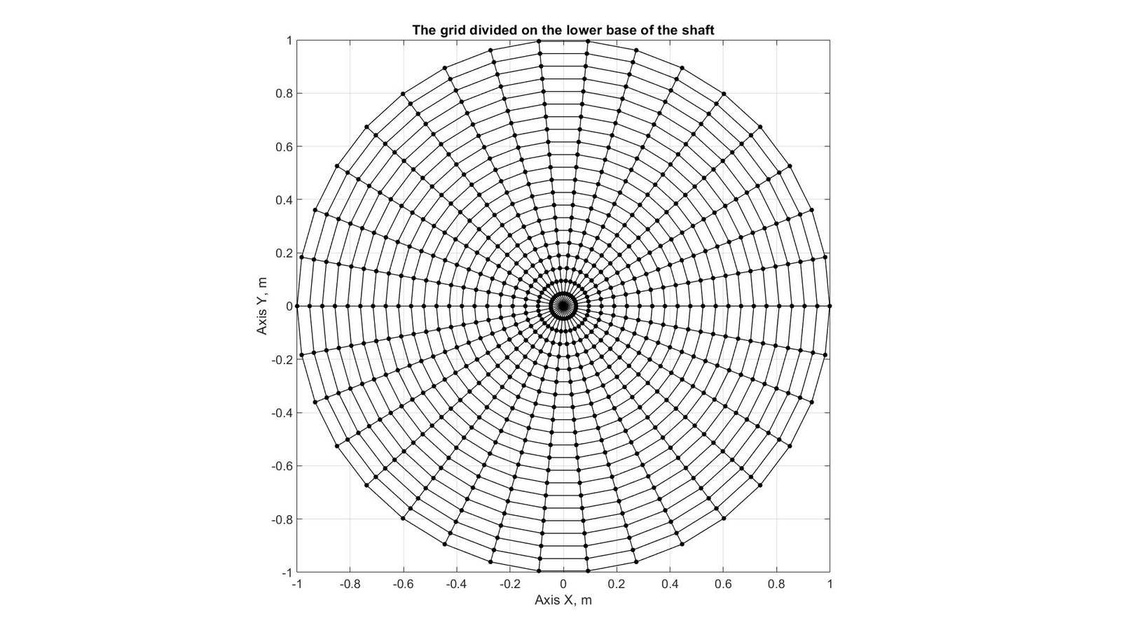
Fig. 3. The grid divided on the lower base of the shaft.
2.4. Calculation of the output luminous flux created by light repeatedly reflected from the inner surface of a light shaft
To calculate the part of the output light flux created by light repeatedly reflected from the inner surface of the shaft, it is necessary to determine the brightness of the beam that comes from the elementary plane on the celestial hemisphere and, after multiple reflections from the inner surface of the shaft, falls into the reference point RP (Fig. 4). Beam brightness \(L_{in}\) at the entrance to the light shaft depends (that follows from brightness distribution models on the firmament) on the angle of its inclination to the horizontal plane (angle \(\theta\)) and the azimuth of its horizontal projection (angle \(\alpha_{in}\)).
Figure 4
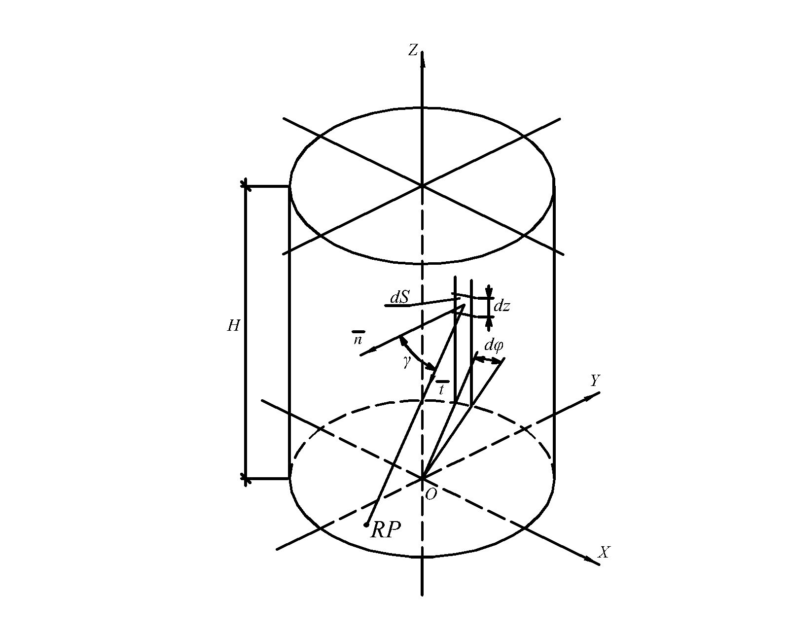
Fig. 4. To determination of illumination by reflected light of the reference point RP of the lower base of the light shaft.
Therefore, it is necessary to determine the angle of inclination \(\theta\) of the input beam to the horizontal plane and the azimuth \(\alpha_{out}\) of its projection onto the same plane using the coordinates of the output beam \(L_{out}\) (they are determined by the coordinates of the reference point RP and the coordinates of the center of the reflecting plane dS). At reflection of the beam from the vertical plane (and the tangent planes to the vertical cylinder of the shaft are vertical), the beam inclination angle to the horizontal plane does not change [36].
Therefore, as we can calculate inclination angle of the output beam, it is necessary to define the number of reflections of the beam Nfrom the internal surface of the shaft to its exit from the shaft. After each reflection of a beam of a given trajectory, the horizontal projection of the beam is rotated by the same angle \(\mathrm{\Delta\phi}\) (clockwise or against it) and falls by the identical size \(\mathrm{\Delta\ z}\) (Fig. 5). The parameters Δφ and Δz for a given beam trajectory are calculated from the coordinates of the reference point RР and the center of the reflecting plane dS. It allows to determine the number of reflections of the beam N to the exit from the light shaft by the formula [36]:
where \(Ent\left(\frac{H-z}{\mathrm{\Delta z}}\right)\) – Antje's function (the integer part of the expression given in brackets); z – z-coordinate of the center of the reflecting plane dS, m; Н – shaft height, m.
Figure 5
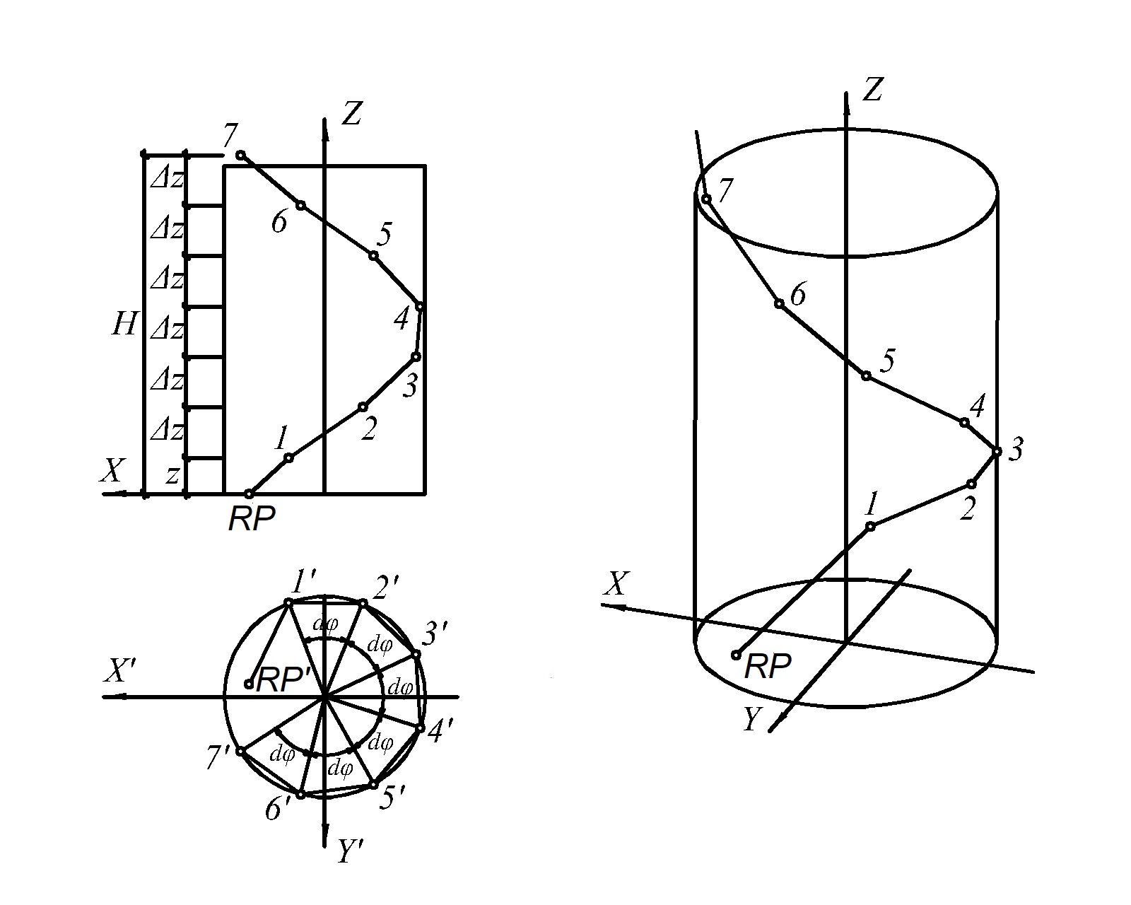
Fig. 5. To determination of number of reflections of light beam from side face of the light shaft (RР-1 – the output beam of the represented trajectory).
In addition, information about the number of beam reflections N allows to determine the azimuth\alpha_{in} of the projection of the entrance beam onto the horizontal plane. All this in total allows to calculate brightness of output beam on formula [36]:
where N – number of reflections of the beam from walls of the light shaft; \(\rho\) – specular reflection coefficient of its inner surface.
Thus, the light vector created in the reference point on the basis of the light shaft by light reflected from the plane is determined by the formula [36]:
Z-coordinate of the light vector created in reference point reflected from all inside face of the shaft, we determine by integration in its limits [36]:
and the module of z-coordinate of light vector is equal to the illumination of the horizontal plane of the lower basis of the shaft in the reference point.
Z-coordinate of light vector and illumination are calculated on the grid of reference points (Fig. 3), divided on the lower base of the light shaft as described above. Then the average value of illumination for each cell is calculated. The output luminous flux \(F_{out}^{ref}\) created by light which is repeatedly reflected from the internal surface of the shaft was calculated similarly i.e. as the sum of the flows passing through each cell.
The block diagram of the entire algorithm for calculating the efficiency of the light shaft is shown in Fig. 6.
Figure 6
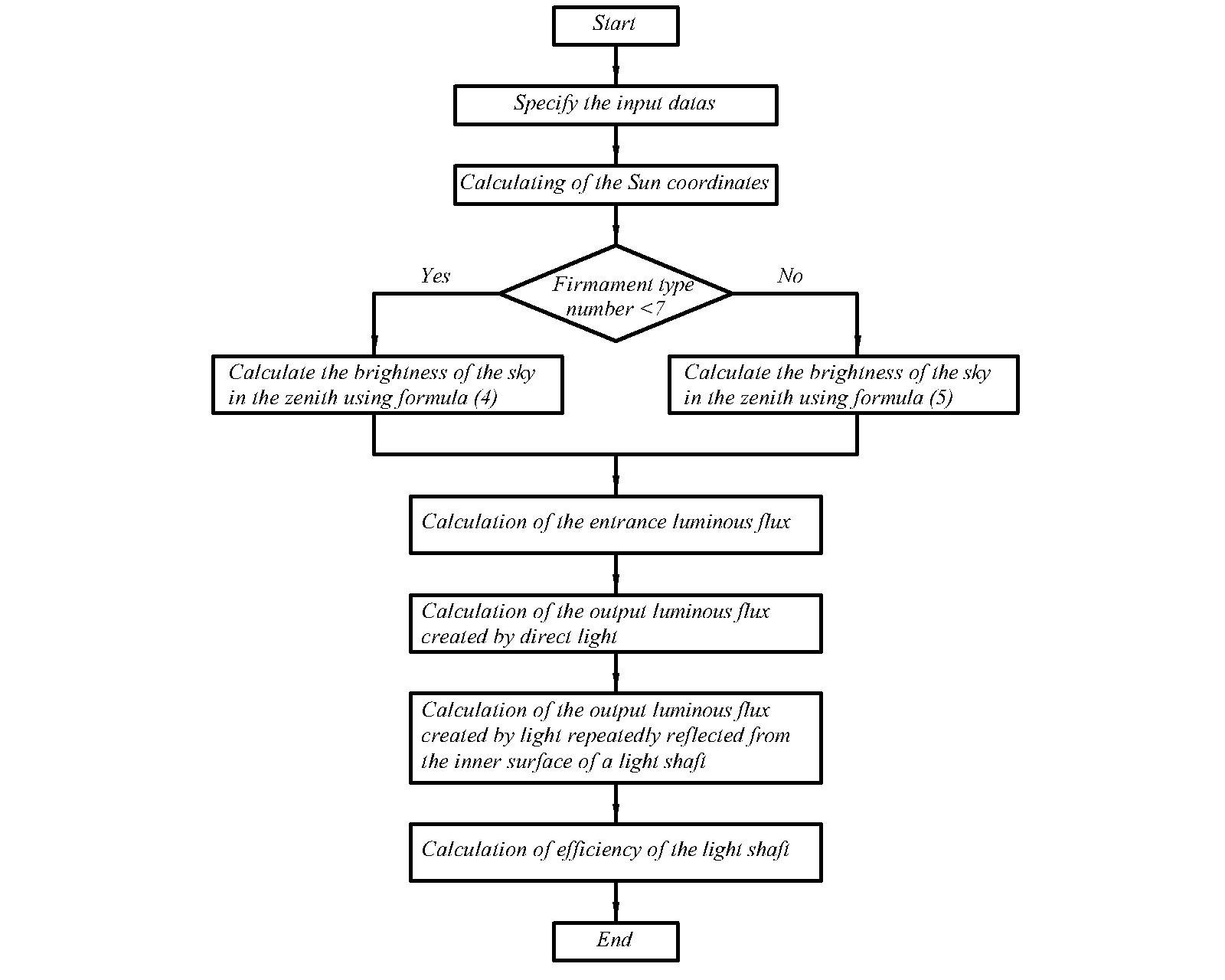
Fig. 6. Block diagram for calculating the efficiency of a light shaft.
3. Сalculation and results
3.1. Input data
Calculation was carried out for the 79th day of year (the vernal equinox: On March 20), the 173rd day of year (summer solstice: On June 22) and the 355th day of year (winter solstice: On December 21). Calculations were carried out for latitude 50o N. The coordinates of the Sun were calculated using well-known formulas [37]:
where \(\gamma_S\) – angular height of the Sun, rad; \(\psi\) – declination of the Sun, rad; \(\omega\) – time angle, rad; \(\varphi\) – latitude, rad.
where \(\alpha_S\) – azimuth of the Sun, rad.
The declination of the Sun is calculated by the formula:
where Nd – day number of the year; \(\psi_m\)=23,45° – the maximum inclination of the Sun.
The time angle associated with solar time \(t_S\) is calculated by the formula:
The solar time of sunrise and sunset was calculated using the formulas:
Solar time is counted from solar noon eastward with a “–” sign, and westward with a “+” sign. Based on the coordinates of the Sun at a certain moment in solar time, the angular distance between an element of the firmament and the Sun was calculated, which is necessary to calculate the brightness of the entering beam.
Duration of sunny day from rising till the sunset for each of the chosen days of year has been separated into 30 equal intervals on which ends the direct and reflected luminous fluxes and efficiency of light shaft for all 15 mathematical models of firmament were calculated. Calculations were carried out in the system of computer mathematics MatLab. Illumination was calculated in kilolux and efficiency as a percentage.
Also, it should be noted that calculations were carried out for different ratios of radius of the shaft to its height \(\frac{R}{H}\), that is for different indexes of the shaft [38-39]. The radius of the shaft was 1 m, and the height of the shaft varied from 0.1111 m to 10 m. It is clear that in architectural and construction practice, light shafts do not use all such ratios, but in order to clearly show the nature of the change in the efficiency coefficient, the calculation was performed for such a wide range.
The entrance luminous flux \(F_{in}\) was calculated on formula (7). For these initial conditions its value was affected by only solar time and type of mathematical model of the firmament.
At calculations of the luminous flux created by the reflected light for integration in the formula (13) the Monte-Carlo method is used [40-42]. It is caused by the fact that determination of number of reflections and trace of beams, demand long-term computer calculations, and use of the Monte-Carlo method considerably reduced their duration. For use of the Monte-Carlo method the field of integration fitted into a unit (in our case two-dimensional) cube by normalizing the parameters \(\phi\in\left[\phi_{op},\phi_{end}\right],z\in\left[z_{op},z_{end}\right]\):
Substituting (20), (21) and (22) into (13), we obtain the limits of integration and parameters expressed in terms of the normalized parameters \(\phi\ast\) and z\(\ast\). Substituting random points in the range of parameters \(\phi\ast\) and z\(\ast\), calculate the integral by the formula:
where M– the total number of the generated points, including those which did not get to the field of integration (in our case all points get to the field of integration as integration happens on all lateral surface of the cylinder); \(f_z^t\)(φ*, z*) – value of integrand function for parameters in random points.
The number of required points is estimated by the formula:
where \(\delta\)– relative accuracy, that is at \(\delta=1\cdot10^{-2},M\geq5\cdot10^3\).
3.2. Results
The analysis of the results received for 15 mathematical models of the firmament showed that they can conditionally be separated into three groups. In the first group of types of the firmament the efficiency of the shaft did not change during the day. In the second group efficiency not strongly changed during the day if not to take into account value for midday. And in the third group the value of efficiency varied during the day and considerably increased at noon. Not to overload article with information, calculation results were given only for two mathematical models of the firmament (one from the second and third groups) – the fourth (overcast, moderately graded and slight brightening towards the Sun) and fifteenth (white-blue turbid sky with broad solar corona).
In Fig. 7, the surface of dependence of total efficiency of the light shaft from solar time and the index of the shaft is shown. Results are received for the fourth type of a firmament and the 79th day of year. The coefficient of light reflection of an internal surface of the shaft \(\rho\) equaled 0.8. Total efficiency of the light shaft at first was calculated for various values of indexes of the shaft and one certain value of solar time. In total these values form the broken flat line which shows dependence of total efficiency of the light shaft on the index of the shaft. Some of these flat polylines (not all, as the polylines merge) are shown in Fig. 8, and Fig. 7 shows the results obtained over the entire sunny day, combined into a surface. It can be seen from Fig. 7 that the values are symmetrical about solar noon. The maximum values correspond to solar noon (from 31.2% to 95.6%), and the minimum values are at sunrise and sunset (from 28.7% to 95.2%). The surface shown in Fig. 7 clearly shows that the total efficiency of the light shaft is almost independent of solar time, and the graphs (Fig. 8) already have more practical significance.
Figure 7

Fig. 7. The surface of dependence of total efficiency of the light shaft from solar time and the index of the shaft (the fourth type of a firmament, the 79th day, reflection coefficient - 0.8).
Figure 8
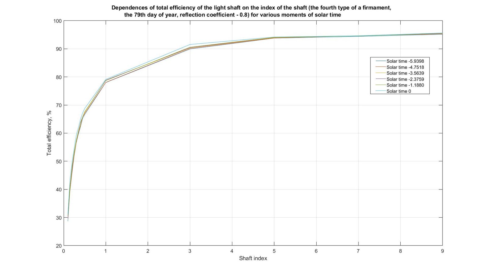
Fig. 8. Dependences of total efficiency of the light shaft on the index of the shaft (the fourth type of a firmament, the 79th day of year, reflection coefficient - 0.8) for various moments of solar time.
In Figs. 9-12 the similar results received for the 173rd and 355th days of year are shown. The nature of the surfaces and curves received for these days is similar to the surfaces and curves received for the 79th day and shown in Figs. 7 and 8. For the 173rd day the maximum values correspond to solar noon (from 34.4% to 96.3%), and the minimum values are at sunrise and sunset (from 29% to 95.2%). For the 355th day, the value at noon is from 29.3% to 96.1%, and at sunrise and sunset – from 29.1% to 95.3%.
Figure 9

Fig. 9. The surface of dependence of total efficiency of the light shaft from solar time and the index of the shaft (the fourth type of a firmament, the 173rd day, reflection coefficient - 0.8).
Figure 10
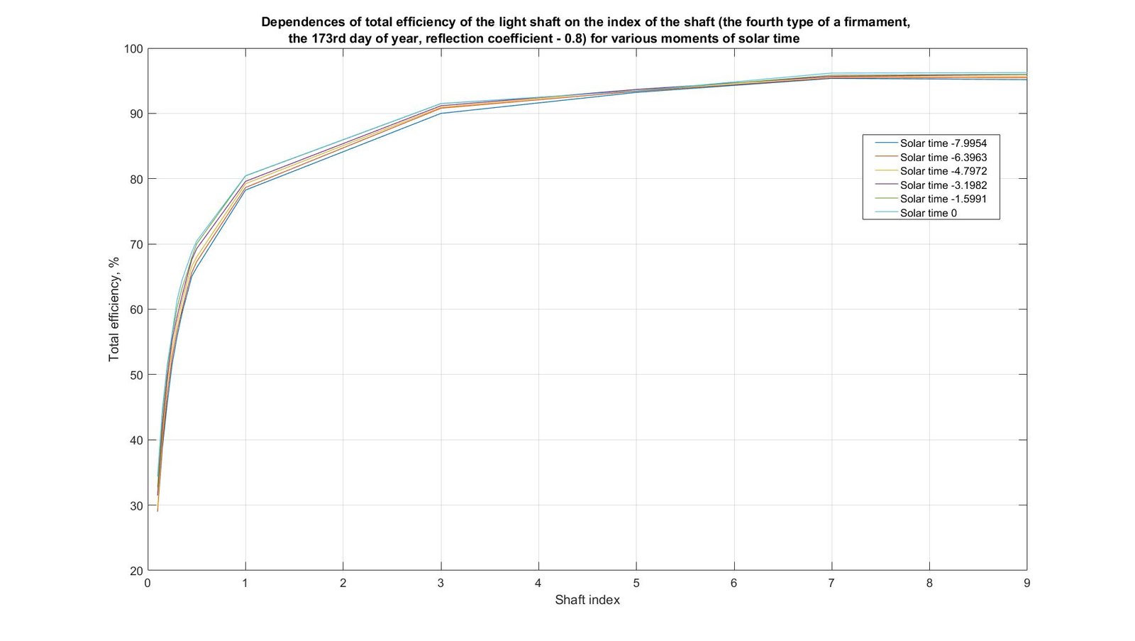
Fig. 10. Dependences of total efficiency of the light shaft on the index of the shaft (the fourth type of a firmament, the 173rd day of year, reflection coefficient - 0.8) for various moments of solar time.
Figure 11
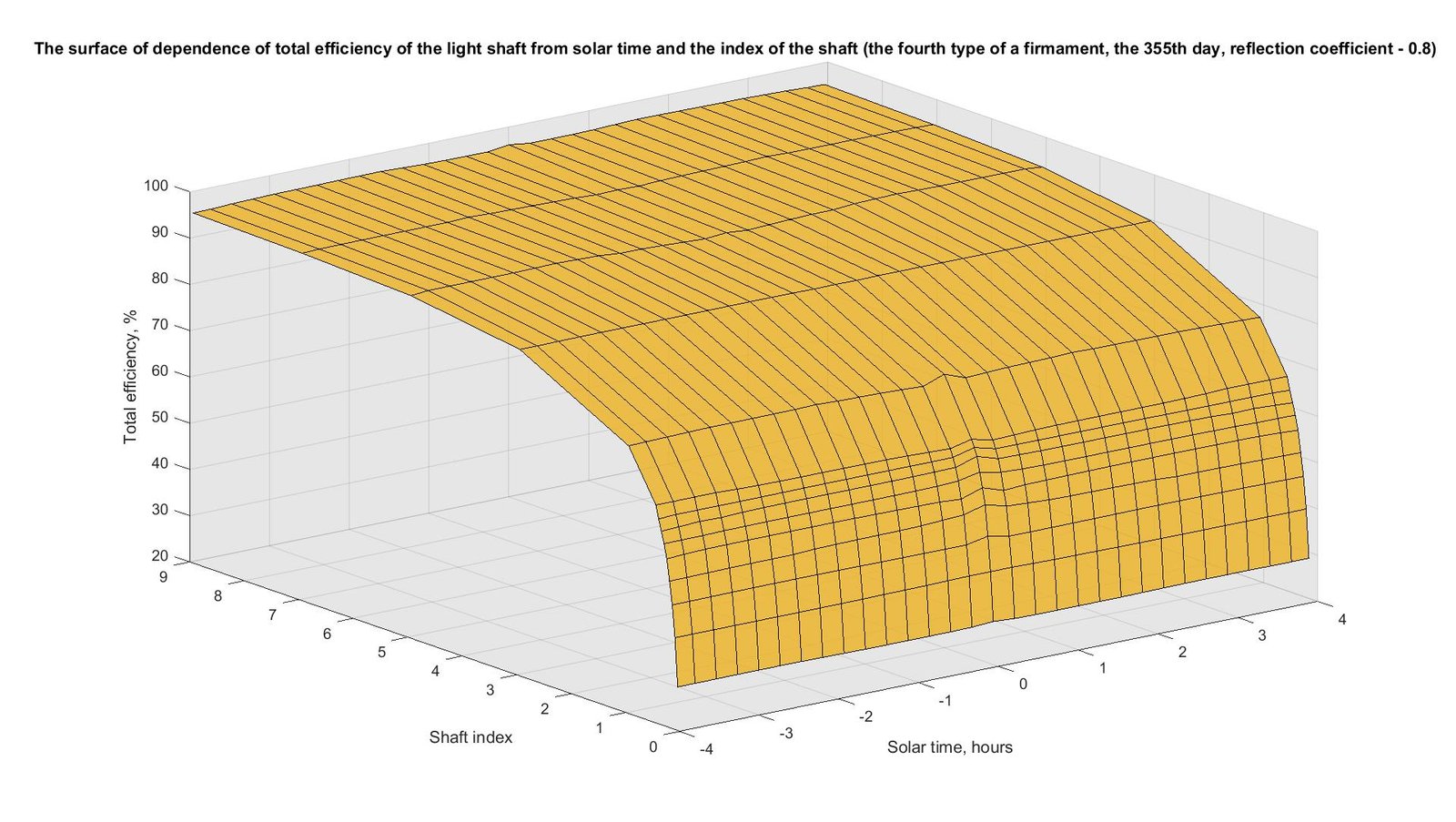
Fig. 11. The surface of dependence of total efficiency of the light shaft from solar time and the index of the shaft (the fourth type of a firmament, the 355th day, reflection coefficient - 0.8).
Figure 12
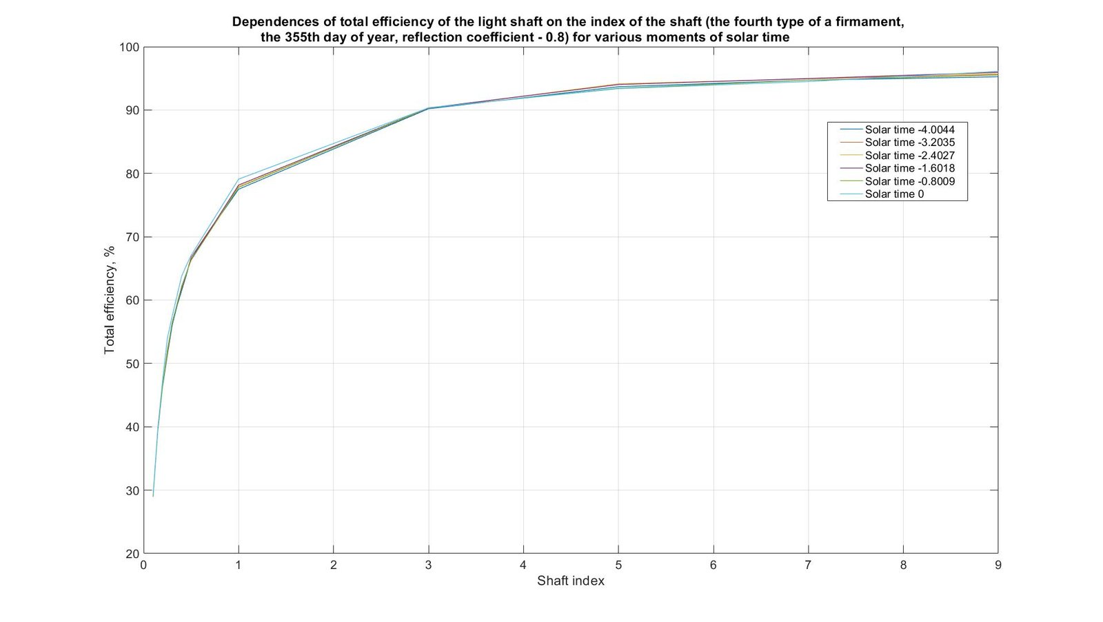
Fig. 12. Dependences of total efficiency of the light shaft on the index of the shaft (the fourth type of a firmament, the 355th day of year, reflection coefficient - 0.8) for various moments of solar time.
In Fig. 13, the surface of dependence of total efficiency of the light shaft from solar time and the index of the shaft is shown. Results are received for the fifteenth type of a firmament, in case of the 79th day of year. The coefficient of light reflection of an internal surface of the shaft \(\rho\) also equaled 0.8. The algorithm for constructing the surface in Fig. 13 and the graphs in Fig. 14 is similar to that in the case of the fourth type of firmament. From Fig. 13, it can be seen that the values are symmetrical about noon. The maximum values were obtained at noon (from 22.7% to 95.4%), and the minimum values were at sunrise and sunset (from 14.1% to 91.2%).
Figure 13
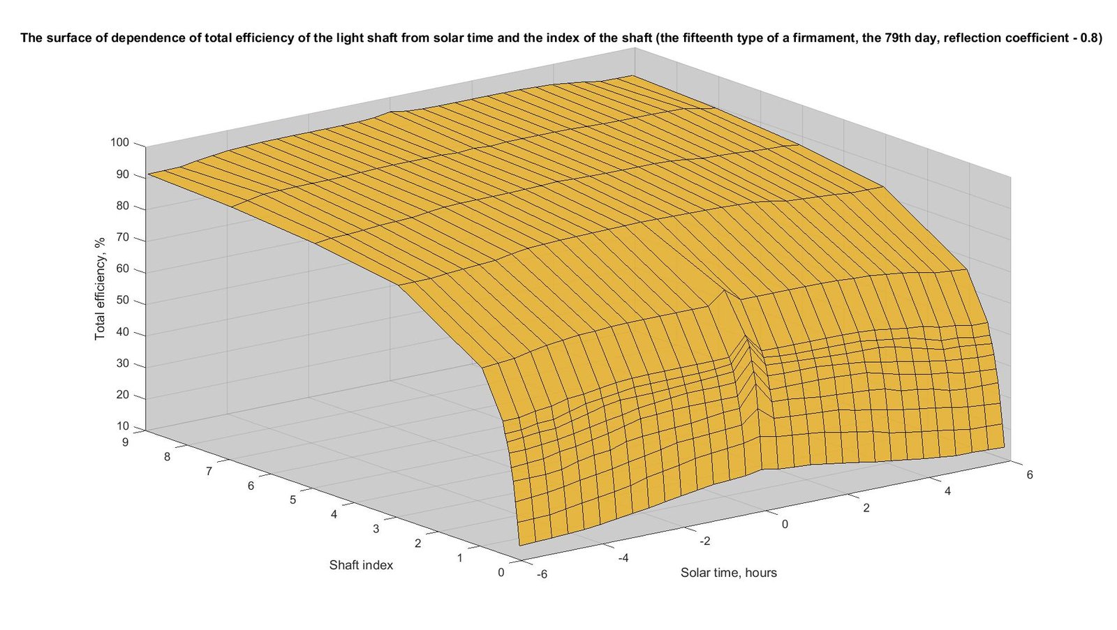
Fig. 13. The surface of dependence of total efficiency of the light shaft from solar time and the index of the shaft (the fifteenth type of a firmament, the 79th day, reflection coefficient - 0.8).
Figure 14
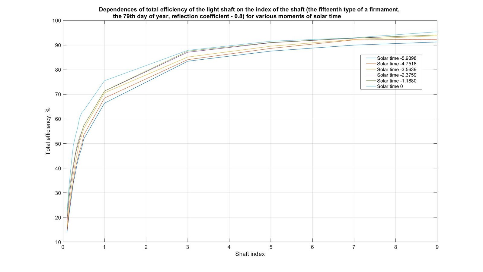
Fig. 14. Dependences of total efficiency of the light shaft on the index of the shaft (the fifteenth type of a firmament, the 79th day of year, reflection coefficient - 0.8) for various moments of solar time.
In Figs. 15-18, the similar results received for the 173rd and 355th days of year are shown. The nature of the surfaces and curves obtained for these days is somewhat different from the nature of the surfaces and curves obtained for the 79th day and shown in Fig. 13-14. For the 173rd day the maximum values correspond to solar noon (from 33.7% to 95.8%), and the minimum values are at sunrise and sunset (from 14.1% to 91.2%). For the 355th day, the value at noon is from 15.5% to 93.4%, and at sunrise and sunset – from 13% to 91.5%. Therefore, this question demands further more detailed research and search of regularities which can practically be used at the solution of various technical tasks.
Figure 15
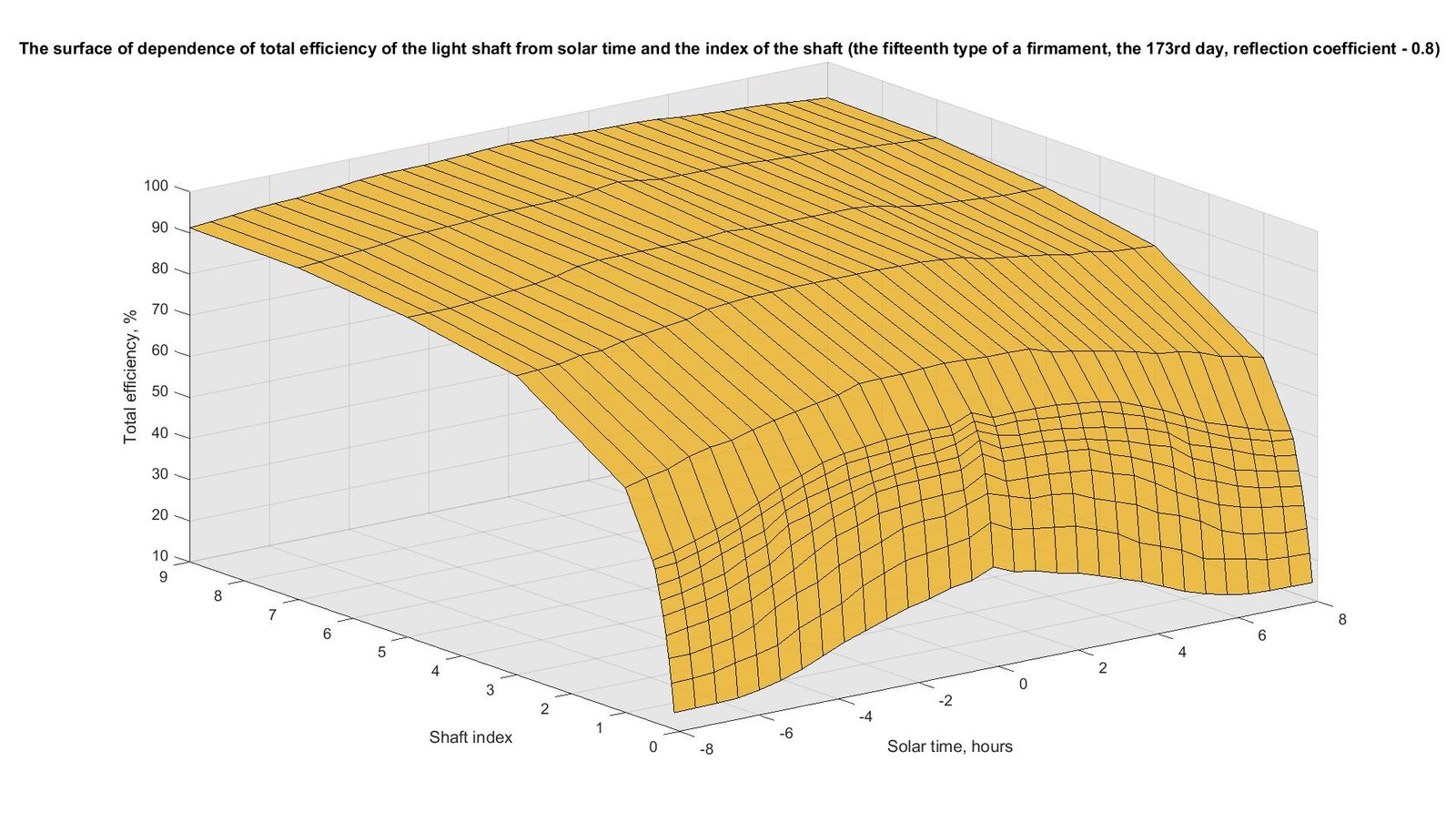
Fig. 15. The surface of dependence of total efficiency of the light shaft from solar time and the index of the shaft (the fifteenth type of a firmament, the 173rd day, reflection coefficient - 0.8).
Figure 16
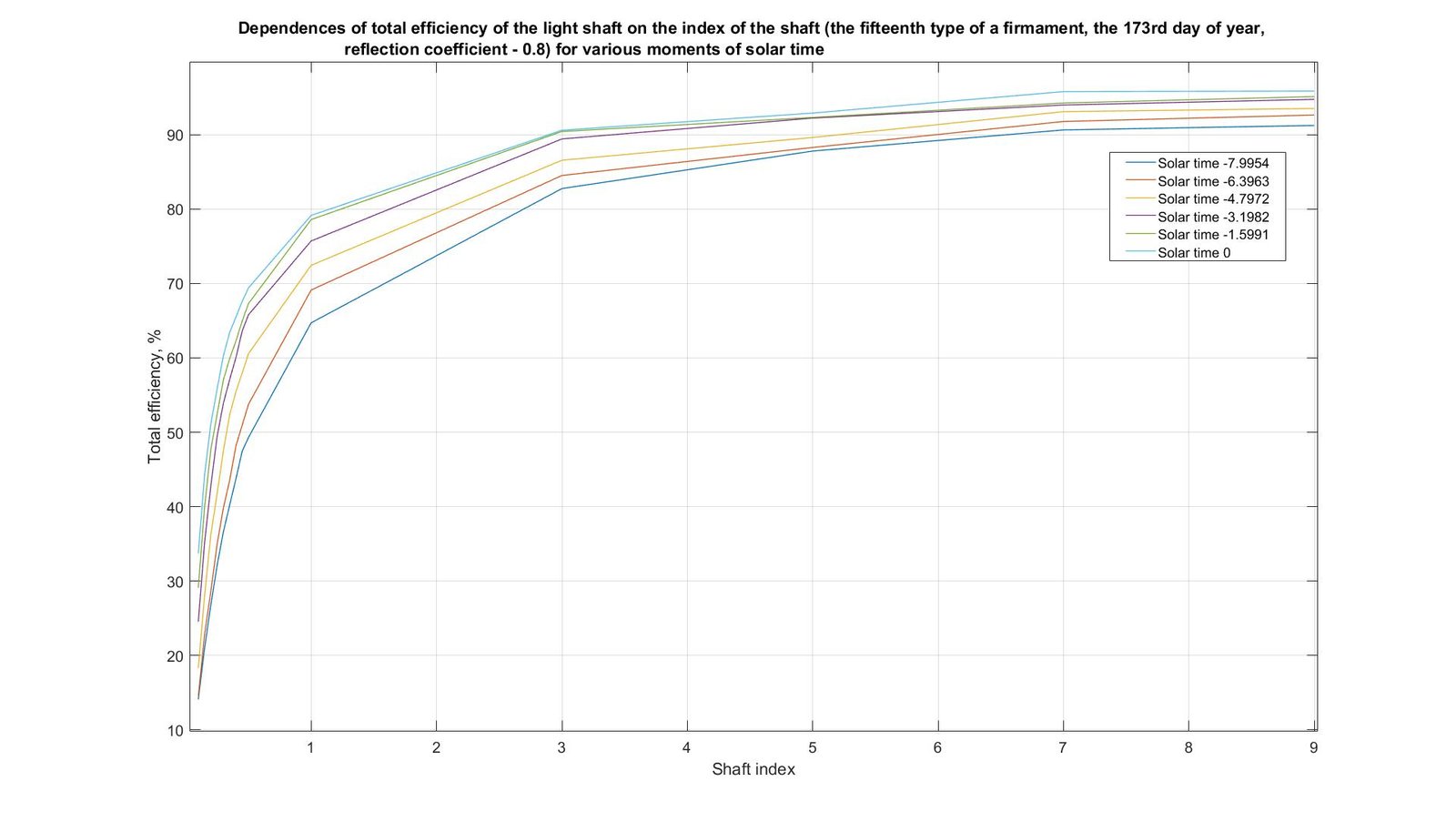
Fig. 16. Dependences of total efficiency of the light shaft on the index of the shaft (the fifteenth type of a firmament, the 173rd day of year, reflection coefficient - 0.8) for various moments of solar time.
Figure 17
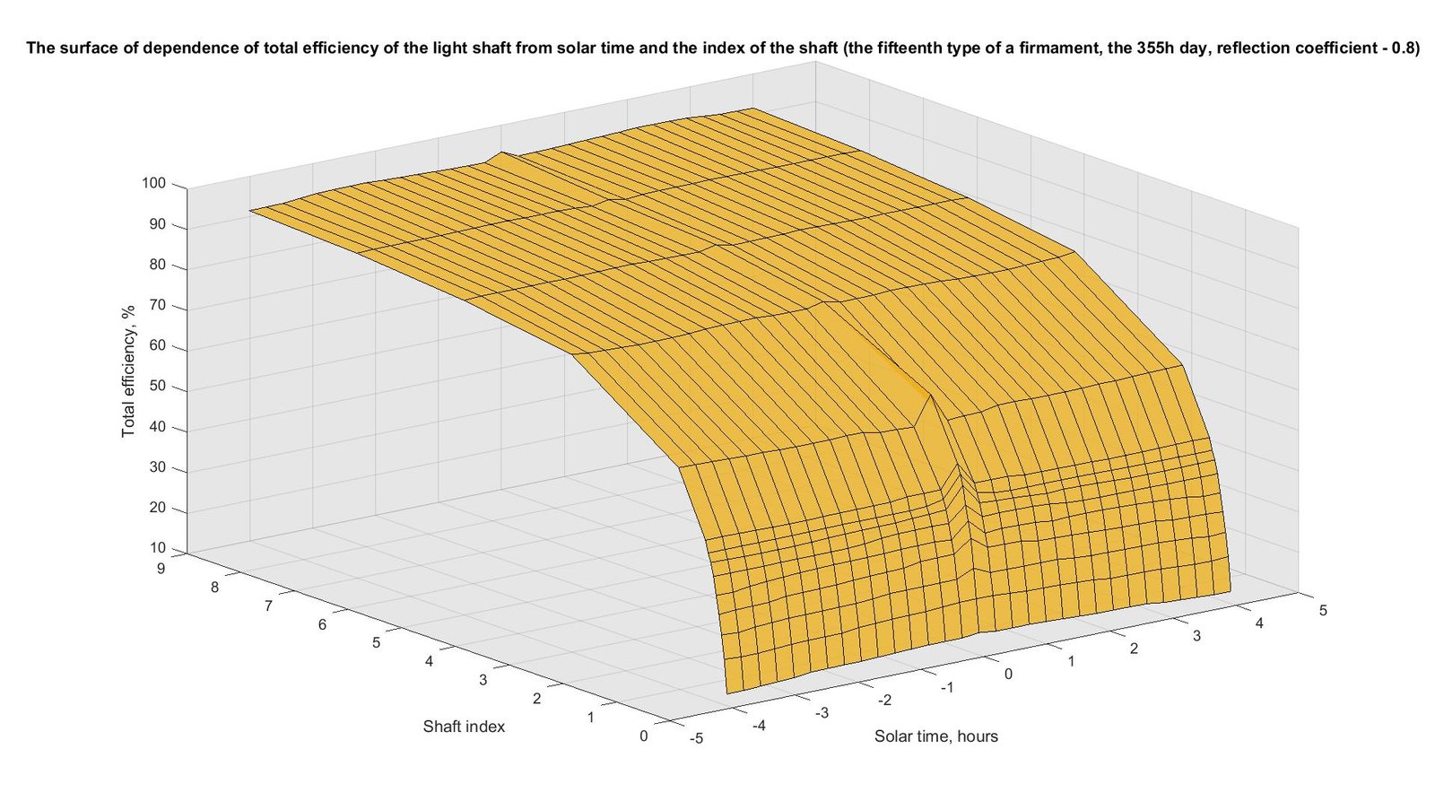
Fig. 17. The surface of dependence of total efficiency of the light shaft from solar time and the index of the shaft (the fifteenth type of a firmament, the 355h day, reflection coefficient - 0.8).
Figure 18
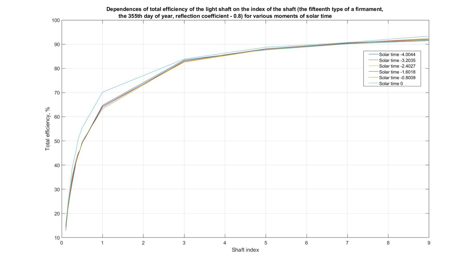
Fig. 18. Dependences of total efficiency of the light shaft on the index of the shaft (the fifteenth type of a firmament, the 355th day of year, reflection coefficient - 0.8) for various moments of solar time.
4. Discussion
Analogous calculations were made for all 15 mathematical models of the firmament. In all cases, as the light shaft index increases, that is, as the ratio \(\frac{R}{H}\) increases, the efficiency value asymptotically approaches one hundred percent, which is physically correct. Knowing R, Hand the shaft index, it is possible to predict natural lighting under the shaft and use energy resources more rationally.
As noted above, in architectural and construction practice, the entire range of shaft indexes involved in calculations is usually not used. Based on an analysis of existing buildings with overhead lighting from light shafts, it was determined that the optimal index of a cylindrical vertical shaft varies from 0.5 to 3 [38-39]. But, if necessary, you can use any of the above light shaft indexes.
However, apparently from Fig. 7-18, the dependence of total efficiency of the light shaft on the index of the shaft for the fourth and fifteenth types of a firmament changes during the day. At noon, the values are maximum, and at sunrise and sunset, they are minimum. These values are affected also by day of year. Results are shown only for two types of a firmament. The remaining thirteen cases also have their own characteristics. For example, for the first type of a firmament (CIE Standard Overcast Sky, Steep luminance gradation towards zenith, azimuthal uniformity) the value of efficiency during the day does not change at all. Therefore, taking into account all of the above, further research and additional analysis are needed.
First, for greater convenience, the graph of the dependence of the total efficiency of the light shaft on the shaft index should be averaged in a certain way. At the same time not to consider value at noon which considerably differs from other values, and value for a certain interval at the beginning and at the end of sunny day, since these are insignificant time intervals compared to the entire solar day.
Secondly, to try to find dependence of change of nature of this average curve within a year. For best accuracy and correctnesses it is necessary to analyse more days of year. Ideal option will be to receive values for every day of year. But because of feature of an algorithm, quite complex calculations, it physically can take a lot of time.
Third, perform similar calculations for other specular reflection coefficient of its inner surface of the shaft. Fourth, perform similar calculations for other geographical latitudes.
It is clear, that for each of 15 mathematical models of a firmament it is necessary to make these researches and the analysis separately.
5. Conclusion
The article considered the issue of determining the efficiency of the vertical specularly reflecting cylindrical light shaft for various types of the firmaments standardized by CIE (International Commission on Illumination). Efficiency of the light shaft was calculated as the relation of the output luminous flux (exiting through the lower base of the shaft) to the entering luminous flux (entering through the upper base of the shaft).
Calculation was carried out for the 79th day of year (the vernal equinox: On March 20), the 173rd day of year (summer solstice: On June 22) and the 355th day of year (winter solstice: On December 21). Calculations were carried out for latitude 50o N. The article directly demonstrates the results for two types of firmament: for the fourth (overcast, moderately graded and slight brightening towards the Sun) and for the fifteenth (white-blue turbid sky with broad solar corona). For the 4th types of firmament the maximum values correspond to solar noon (from 29.3% to 96.3%), and the minimum values are at sunrise and sunset (from 28.7% to 95.3%). For the 15th types of firmament the maximum values correspond to solar noon (from 15.5% to 95.8%), and the minimum values are at sunrise and sunset (from 13% to 91.5%).
Therefore, it can be argued that solar time has little effect on the efficiency, which allows us to generalize the results obtained in a certain way. For example, we can calculate the arithmetic mean value during the day, but ignore the value at noon, which is significantly different from other values, and the value for a certain interval at the beginning and end of the solar day, since these are insignificant time intervals compared to the entire solar day.
The results also showed that as the light shaft index increases, that is, as the ratio of the radius to the shaft height increases, the efficiency value asymptotically approaches one hundred percent, which is physically correct. Information on the radius, height, index of the shaft and the specular reflection coefficient of its inner surface allows to predict natural illumination under the shaft, rationally use artificial lighting, saving on it.
In addition, the developed MatLab program can be used to simulate natural lighting in rooms of buildings of various purposes from light shafts of various sizes.
Further research can be directed at modeling natural light from light shafts of other geometric shapes (e.g., rectangular or conical) or light shafts with diffuse light reflection.
Contributions
S. Litnitskyi: Conceptualization, Writing-original draft, Visualization, Investigation, Software, Data curation, Writing- review & editing. E. Pugachov: Conceptualization, Writing- review & editing. T. Kundrat: Formal analysis. V. Zdanevych: Formal analysis.
Funding
This research received no external funding.
Declaration of competing interest
The authors declare no conflict of interest.
References
- CIE S 003/E:1996 (ISO 15469:1997) «CIE standard overcast sky and clear sky».
- CIE S 011/E:2003 (ISO 15469: 2004(E). «Spatial distribution of daylight - CIE standard general sky».
- DSTU ISO 15469:2008. «Spatial daylight brightness distribution. CIE standard cloudy and cloudless sky (ISO 15469:2004, IDT)». (in Ukrainian)
- K. Alshaibani, Average Daylight Factor for the ISO/CIE Standard General Sky, Lighting Res. Technol. 48 (2016) 742-754.
- R. Kittler, S. Darula, CIE General Sky Standard Defining Luminance Distribution, Proceedings of eSim Conference. Montreal, Canada (2002) 36-43.
- R. Kittler, S. Darula, The Research Search for the Least Beneficial Overcast Sky and Progress in Defining Its Luminance Gradation Function, Building Research Journal 61 (2014) 151-166. https://doi.org/10.2478/brj-2014-0012
- W. Li, L. Tang, M. Lee and T. Munner, Classification of CIE Standard Skies Using Probabilistic Neural Networks, International Journal of Climatology 30 (2009) 305-315. https://doi.org/10.1002/joc.1891
- P. R. Tregenza, Analysing Sky Luminance Scans to Obtain Frequency Distributions of CIE Standard General Skies Generation Communication and Networking (25-28 November 2015, Jeju Island, South Korea), FGCN 2015 IEEE CPS Post Proceedings. Jeju: SERSC, 49-54.
- Yu-Feng Ho Aggression Models for the Indoor Natural Lighting in House Building. Thesis for the Degree of Master. Chaoyang University of Technology, 2012.
- D. H.W. Li, T.C. Chau, K. K.W. Wan, A Review of the CIE General Sky Classification Approaches, Renewable and Sustainable Energy Reviews, 31 (2014) 563-574. https://doi.org/10.1016/j.rser.2013.12.018
- D. Radomtsev, O. Sergeychuk, Implementation of CIE General Sky Model Approach in Ukraine and Effects on Room Illuminance Mode, International Journal of Smart Home. Tasmania: SERSC, 10 (2016) 57-70. https://doi.org/10.14257/ijsh.2016.10.1.07
- D. Radomtsev, O. Sergeychuk, Employment Features of CIE S 011/E:2003 (ISO 15469: 2004) "CIE Standard General Sky" under Designing Systems of Room Daylighting. 9th International Conference on Future Technology 39 (2007) 31-51.
- S. K. Wittkopf, Analysing Sky Luminance Scans and Predicting Frequent Sky Patterns in Singapore, Lighting Research and, Lighting Research and Technology 36 (2004) 271-281. https://doi.org/10.1191/1477153504li117oa
- M. B. Piderit, C. Cauwerts, M. Diaz, Definition of the CIE Standard Skies and Application of the HDRI Technique to Characterize the Spatial Distribution of Daylight in Chile, Journal of Construction 13 (2014) 22-30. https://doi.org/10.4067/S0718-915X2014000200003
- E. Ng, V. Cheng, A. Gadi, J. Mu, M. Lee and A. Gadi, Defining Standard Skies for Hong Kong, Building and Enviroment 42 (2007) 866-876. https://doi.org/10.1016/j.buildenv.2005.10.005
- E. V. Pugachev, S. I. Litnitskyi, T. M. Kundrat, V. A. Zdanevych, Definion Analysis of the Ratio of the Luminance in an Arbitrary Sky Elements to the Zenith Luminance Given in DSTU ISO 15469:2008, Modern Problems of Modeling 25 (2023) 184-192. https://doi.org/10.33842/2313-125X-2023-25-184-192
- M. Kocifaj, F. Kundracik, S. Darula and R. Kittler, Theoretical Solution for Light Transmission of a Bended Hollow Light Guide, Solar Energy 84 (2010) 1422-1432. https://doi.org/10.1016/j.solener.2010.05.002
- I. Acosta, J. Navarro, J. J. Sendra, Lighting Design in Courtyards: Predictive Method of Daylight Factors under Overcast Sky Conditions, Renewable Energy 71 (2014) 243-254. https://doi.org/10.1016/j.renene.2014.05.020
- M. Kocifaj, S. Darula, R. Kittler, HOLIGILM: Hollow Light Guide Interior Illumination Method - An Analytic Calculation Approach for Cylindrical Light-Tubes, Solar Energy 82 (2008) 247-259. https://doi.org/10.1016/j.solener.2007.07.003
- R. Kittler, M. Kocifaj, S. Darula, Daylight Science and Daylighting Technology, New York, Springer, 2012. https://doi.org/10.1007/978-1-4419-8816-4
- D. Phillips, Daylighting. Natural Light in Architecture, Elsevier, 2004.
- T. M. Kundrat, Geometric Modeling of Lighting from Light Shafts with Diffuse Light Reflection, NUWEE PhD dissertation, 2010. (in Ukrainian)
- M. Kocifaj, F. Kundracik, S. Darula and R. Kittler, Availability of Luminous Flux below a Bended Light-Pipe: Design Modelling under Optimal Daylight Conditions, Solar Energy 86 (2012) 2753-2761. https://doi.org/10.1016/j.solener.2012.06.017
- H. von Wachenfelt, V. Vakouli, A. P. Diéguez', N. Gentile, M.-C. Dubois and K.-H. Jeppsson, Lighting Energy Saving with Light Pipe in Farm Animal Production, Journal of Daylighting 2 (2015) 21-31. https://doi.org/10.15627/jd.2015.5
- A. P. Diéguez', N. Gentile, H. von Wachenfelt and M.-C. Dubois, Daylight Utilization with Light Pipe in Farm Animal Production: A Simulation Approach, Journal of Daylighting 3 (2016) 1-11. https://doi.org/10.15627/jd.2016.1
- B. Obradovic, B. S. Matusiak, Daylight Transport Systems for Buildings at High Latitudes, Journal of Daylighting 6 (2019) 60-79. https://doi.org/10.15627/jd.2019.8
- A. Goharian, M. Mahdavinejad, A Novel Approach to Multi-Apertures and Multi-Aspects Ratio Light Pipe, Journal of Daylighting 7 (2020) 186-200. https://doi.org/10.15627/jd.2020.17
- P. Zazzini, A. Di Crescenzo, R. Giammichele, Daylight Performance of the Modified Double Light Pipe (MDLP) Through Experimental Analysis on a Reduced Scale Model, Journal of Daylighting 9 (2022) 164-176. https://doi.org/10.15627/jd.2022.13
- B. Obradovic, B. S. Matusiak, Illumination and Lighting Energy Use in an Office Room with a Horizontal Light Pipe: Field Study at a High Latitude, Journal of Daylighting 9 (2022) 209-227. https://doi.org/10.15627/jd.2022.16
- P. Zazzini, A. Di Crescenzo, L. Pio Rossitti, R. Mirando, Experimental Analysis on a 1:2 Scale Model of the Modified Double Light Pipe, Journal of Daylighting 9 (2022) 228-241. https://doi.org/10.15627/jd.2022.17
- N. Sönmez, A. C. Kunduracı, C. Çubukçuoğlu, Daylight Enhancement Strategies Through Roof for Heritage Buildings, Journal of Daylighting 11 (2024) 234-246. https://doi.org/10.15627/jd.2024.17
- Apple Store Fifth Avenue / Foster + Partners. [Online]. Available: https://www.archdaily.com/925305/apple-store-fifth-avenue-foster-plus-partners (accessed Apr. 15, 2025).
- Rooflight F100 Circular (LAMILUX). [Online]. Available: https://www.archdaily.com/catalog/us/products/23868/rooflight-f100-circular-lamilux?ad_source=neufert&ad_medium=gallery&ad_name=close-gallery (accessed Apr. 15, 2025).
- R. Kittler, R. Perez, S. Darula, A Set of Standard Skies Characterizing Daylight Conditions for Computer and Energy Conscious Design. Final report of the U.S.-Slovak Grant project US-SK 92 052, Bratislava, Polygrafia, 1998.
- EN 12665:2002 Light and lighting - Basic terms and criteria for specifying lighting requirements, Management Centre: rue de Stassart, Brussels.
- Yu. V. Garbaruk, Geometric Modeling of Daylighting from Specularly Reflecting Light Shafts, NUWEE PhD dissertation, 2016. (in Ukrainian)
- I. A. Duffie, W. A. Beecman, Solar Energy Thermal Processes, New York-London-Sydney-Toronto, A Wiley-Intercience Publication, 1974.
- Yu. V. Garbaruk, T. M. Kundrat, E. V. Pugachev, The Influence of the Reflectance Coefficient on the Efficiency of Cylindrical Light Shafts, Energy Saving in Construction 1 (2011) 62-67. https://repositary.knuba.edu.ua/items/39945375-1248-48a1-8225-7a9a38e3bd20 (in Ukrainian)
- Yu. V. Garbaruk, T. M. Kundrat, E. V. Pugachev, Comparison of the Efficiency of Cylindrical Light Shafts with Diffuse and Specularly Reflection of Light, Technical Aesthetics and Design 8 (2010) 75-79. (in Ukrainian)
- N. Metropolis, S. Ulam, The Monte Carlo Method, J. Amer. statistical assoc. 44 № 247 (1949) 335-341. https://doi.org/10.1080/01621459.1949.10483310
- A. Doucet, N. de Freitas, N. Gordon, Sequential Monte Carlo Methods in Practice, New York, Springer, 2001. https://doi.org/10.1007/978-1-4757-3437-9
- G. S. Fishman, Monte Carlo: Concepts, Algorithms, and Applications, New York, Springer, 1995.
2383-8701/© 2025 The Author(s). Published by solarlits.com. This is an open access article distributed under the terms and conditions of the Creative Commons Attribution 4.0 License.

1944
Total views
Citations
SHARE ON


