Metamodeling of the Energy Consumption of Buildings with Daylight Harvesting – Application of Artificial Neural Networks Sensitive to Orientation

*Corresponding author. Tel: +55 (48) 37217080; Web: http://www.labcon.ufsc.br
raphaela.walger@ufsc.br (R. W. da Fonseca)
ruttkay.pereira@ufsc.br (F. O. R. Pereira)

History: Received 16 July 2021 | Revised 23 August 2021 | Accepted 31 August 2021 | Published online 06 November 2021

Citation: Raphaela Walger da Fonseca, Fernando Oscar Ruttkay Pereira, Metamodeling of the Energy Consumption of Buildings with Daylight Harvesting – Application of Artificial Neural Networks Sensitive to Orientation, Journal of Daylighting 8 (2021) 255-269. https://dx.doi.org/10.15627/jd.2021.20

Figures and tables

Figure 1
Figure 2
Figure 3
Table 1
Table 2
Table 3
Table 4
Figure 4
Figure 5
Figure 6
Figure 7
Figure 8
Figure 9
Figure 10
Figure 11

Abstract

Daylight harvesting is a well-known strategy to address building energy efficiency. However, few simplified tools can evaluate its dual impact on lighting and air conditioning energy consumption. Artificial neural networks (ANNs) have been used as metamodels to predict energy consumption with high precision, few input parameters and instant response. However, this approach still lacks the potential to estimate consumption when there is daylight harvesting, at the ambient level, where the effect of orientation can be noted. This study investigates this potential, in order to evaluate the applicability of ANNs as a tool to aid the architectonic design. The ANNs were approached as metamodels trained based on EnergyPlus thermo-energetic simulations. The network configuration focused on determining its simplest feasible form. The input parameters adopted as the main variables of the building envelope were as follows: orientation, window-to-wall ratio and visible transmission. The effects of the encoding of orientation as a network input parameter, the number of examples of each variable for network training and changing the parameters used for the training were evaluated. The networks predicted the individualized consumption according to the end use with errors below 5%, indicating their potential to be applied as a simplified tool to support the design process, considering the elementary variables of the building envelope. The discussion of results focused on guidelines and challenges to achieve this purpose when contemplating the broadening of the metamodel scope.

Keywords

Daylight harvesting, Energy consumption, Metamodels, Artificial neural networks

1. Introduction

Daylight is a renewable resource and it can be used in order to save electrical energy in buildings [1,2]. Even with the advent of light-emitting diodes (LEDs), lighting is still responsible for around a third to an eighth of the energy consumption in residential buildings and a third in commercial constructions [3]. In the case of commercial buildings, where control strategies are more easily applied, the potential for daylight harvesting is reinforced by the business schedule coinciding with the availability of daylight [4,5]. However, for the optimization of its use, the designer must make the appropriate decisions in the design conception [6]. Decisions related to the orientation and dimensioning of the openings are fundamental for the success of daylight harvesting strategies implemented in the design stage [7]. Thus, the designers need to be provided with reliable tools to aid them in the beginning of the designing process when information is still scarce. The main challenge associated with these tools is considering the dual impact of daylight harvesting on the lighting and air conditioning energy consumption.

In recent decades, the evolution of technological has impacted the development of computer resources for the evaluation of the energy performance of buildings [8,9]. This has enabled complex thermo-energetic simulations to be carried out more efficiently allowing, as a result, the development of simplified tools based on these simulations [10-14]. In general, tools based on pre-simulated cases are divided into applications with graphic interfaces [10,11] and metamodels based on statistical [13-16] or computational techniques, such as the artificial intelligence [17-19].

Regarding the applicability of this class of tools, the freedom in the definition of the input parameters is restricted to the range of the pre-simulated set; however, they deliver instantaneous responses and do not require specialized expertise. The main advantage is that they originate from the simulation of the annual thermo-energy, based on the climate, and thus the total effect of daylight harvesting is considered. This is because they consider the balance between light and heat originating from openings, along with the variation in the heat dissipated by lamps depending on their use according to the availability of natural light [20].

In this context, studies on metamodels aimed at estimating the energy performance of buildings have increased [21-24]. On a smaller scale, there are studies in which daylight harvesting has been incorporated [25-27]. Regarding daylight, there are applications regarding operation of shading devices [28], of lighting system [29] and prediction of daylight sufficiency [30] based on illuminance simulations. Several techniques which make use of artificial intelligence (AI) have been employed for the metamodeling of energy performance, and many of these involve the use of artificial neural networks (ANNs) [31,32]. ANNs are computational techniques inspired on biological neural networks with a nonlinear approach where AI is employed to represent or approximate systems [33]. These techniques have also been considered promising for the modeling of the energy and lighting performance of buildings, based on measured data [34]. In the context of natural lighting, this modeling type is usually employed in order to estimate luminance [35].

Notable abilities of ANNs are that they can be used to model nonlinear functions, allow a high degree of generalization, require only small amounts of initial information and provide fast responses. However, a significant challenge associated with their application is that they are ‘black box’ models, and their internal structure is unknown [36]. ANNs are comprised of interconnected neurons and their learning is correlated to the synaptic adjustment process. It is because of this process that they are characterized as black box models. Thus, their optimization is limited to the analysis of the relation between their inputs and outputs as well as their architecture and training parameters [37]. When applied as a metamodel, it is important to evaluate the capacity of the ANN to carry out elementary tasks of computational simulation, to ensure the reliability of the results [36].

On reviewing the literature, it can be noted that there is a lack of studies on the potential use of ANNs to estimate the impact of daylight harvesting on the energy consumption taking into account the effect of orientation. This is because most authors carried out simulations using the traditional “core and shell” thermo model, where consumption is based on the 5 grouped thermo zones, thus, the ANNs were trained with the sum of data from all of them, not allowing to verify the sensitivity of the networks to the effect of each one of them individually [25]. This mitigates the influence of orientation, which is fundamental for the performance of natural lighting. This leads to an important limitation in our knowledge regarding the potential of applying ANNs to obtain estimates involving daylighting. Differently from thermal analysis, daylight analysis takes place at the environment level, so it is essential that a simplified tool aimed at estimating the potential for using daylight to save energy is sensitive to the impact of the orientation of the environment openings. Buildings located in the urban fabric usually have larger openings on the main facades, facing the streets, and smaller ones on the facades facing the other boundaries of the site, as the sides and the rear. The shape of the building and its implementation on the site can also mean that certain orientations present greater potential for taking advantage of daylight than others. As an example, Fig. 1 shows two commercial buildings with similar built-up areas and their main façades face the same street. However, their potential for daylight harvesting varies depending on the area of the façade openings and their respective orientations.

Figure 1

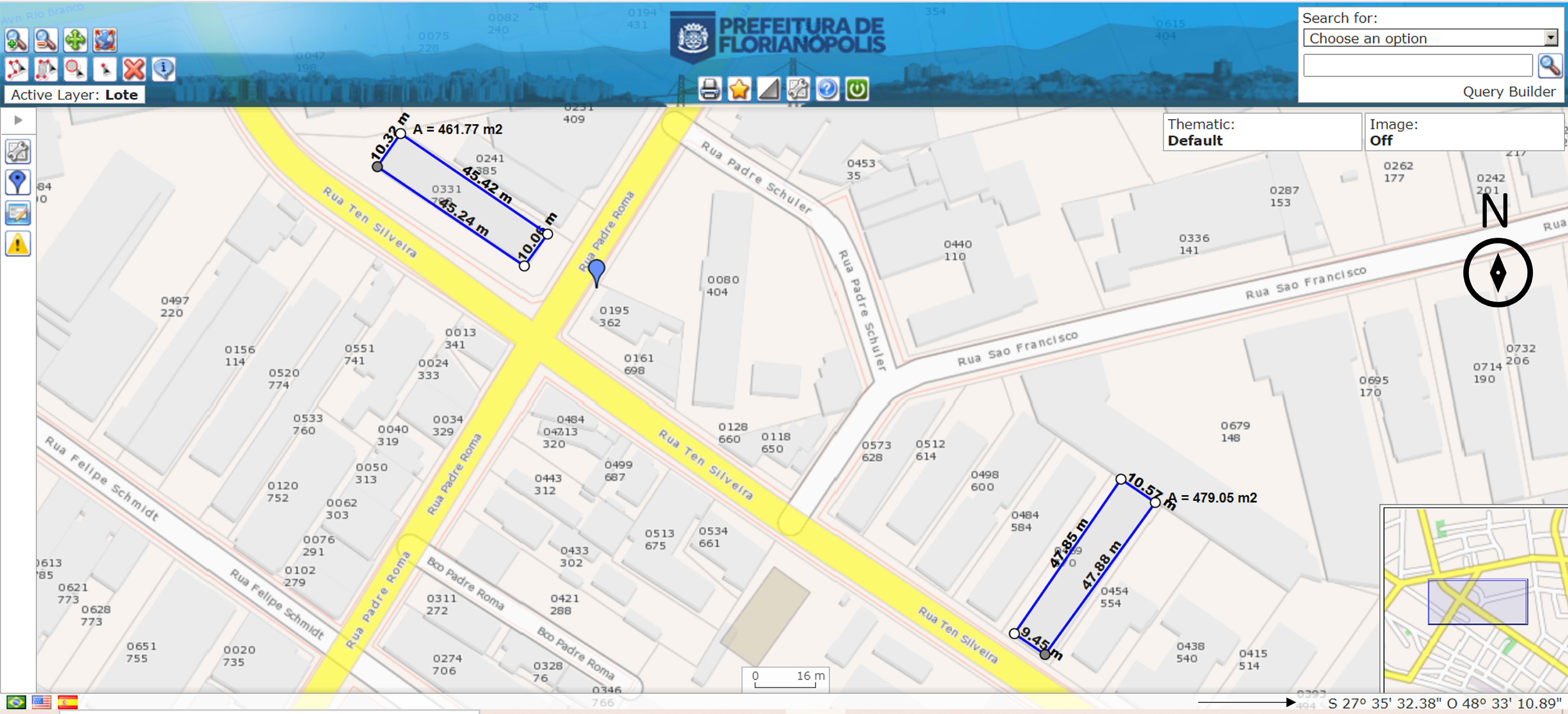
Fig. 1. Example of similar buildings for which the daylighting performance is altered by orientation.

Moreover, the studies in which only one thermal zone was adopted present limitations regarding the test method, since the accuracy of the networks was verified employing a percentage of the parametric dataset. Although this constitutes a novel combination, the variable values had been previously presented to the network [38]. Thus, in the study reported herein, ANNs were investigated with regard to their potential use in the metamodeling of the energy consumption of buildings with daylight harvesting, at the ambient level, where the influence of orientation can be noted.

This work forms part of the development process aimed at obtaining a simplified tool to assist architects in decision making in the early stages of a design project. The content of this article forms the basis for this development process and can be extended to other ANN applications involving daylighting. At this stage, the aim was to investigate the sensitivity of ANNs with regard to modeling the effect of orientation on energy consumption when there is daylight harvesting, elucidating important aspects of their configuration and the generation of the database for their training. In the context of developing a simplified tool, the results reported herein could serve as a basis for the development of other more complex models, with scopes encompassing formal, constructive and building context aspects. Once trained, ANNs can be used easily through a web interface, where inputs are typed in and outputs are returned instantly, enabling its use by professionals with different degrees of expertise.

2. ANNs as metamodels

Artificial neural networks trained with data obtained through simulation are referred to as metamodels because they are computational models based on other models, i.e., those used by the simulation program [40,41]. In thermo-energetic simulation, mathematical and statistical models based on the observation of the physical phenomenon are used, which relate input and output data. The most widely used metamodels make use of empirical regression, where the constants attributed to the independent variable in order to generate a dependent variable are obtained through multivariable regression, applying statistical models [15]. Similarly, for the ANNs, the generation of these constants (the weights) arises from relations between stimuli and targets, uses computational models and occurs through a nonlinear combination of these stimuli. The weights are defined through synaptic adjustment between neurons and will be dependent on the architecture and training configurations of the network.

The basic structure of an ANN is the neuron. Haykin [33] defines the artificial neuron as a mathematically simple processing unit, since it receives one or more inputs, which have an associated synaptic weight, and transforms them into outputs. The neuron is comprised of a summation function¹, responsible for the effective input calculation for the neuron and an activation function², which transmits the output signal. Initially, the synaptic weights are randomly defined and are adjusted according to the learning algorithm³. The knowledge of the network is represented by synaptic weights, which determine the importance of each input. The influence that each input will have on the output increases according to the degree to which the synaptic connection is stimulated⁴.

Synapses are characterized by a weight (w), which is initially random, and this represents its intensity (Fig. 2). The weight wkj multiplies the signal xj, at the input of the synapse j, connected to the neuron k. The result of this operation is submitted to a threshold (θ), which is associated with the activation function. The type of activation is selected in such a way that it softens the updating of the weights [42]. The threshold is fundamental, since it defines whether or not the signal will be propagated. If the ʋk value is higher than the threshold, the weight wkj will be positive and the neuron will be active (excitatory action) and if it is lower than the threshold, the signal will be negative and the neuron output will remain inhibited (inhibitory action).

Figure 2

Fig. 2. Multilayer perceptron neural network: error backpropagation algorithm.

The way in which neurons are structured in the neural network is strongly related to the learning algorithm employed to train it [33]. The learning algorithms determine the rules to be applied for the learning process. There are several typologies of ANNs; however, they can be grouped into two basic classes: (i) non-recurrent and (ii) recurrent [42]. The non-recurrent ANNs are said to be “without memory” because they do not have re-feeding of their outputs to their inputs. These ANNs are structured in one or more layers. Multi-layer feed forward networks are distinguished by the presence of hidden layers. Their function is to intervene in a useful way between the input and output of the network, enabling the extraction of high order statistics⁵ [33].

The network architecture adopted in this study was non-recurrent and feedforward through multiple layers with the adoption of the multilayer perceptron (MLP). The size of an MLP ANN is determined empirically and the heuristic adopted should consider the power of convergence and the generalization of the network [48]. The learning process applied to MLP networks is supervised and the error backpropagation algorithm is used, as seen in Fig. 2 [33].

The error backpropagation algorithm is based on a learning rule which seeks to correct the error during the training phase, originally the delta rule or gradient descent. Its action consists of two steps through different ANN layers: propagation and backpropagation. As described by Haykin [33], during propagation a pattern of activity is applied to the sensor nodes of the network and the effect propagates layer by layer, producing a set of outputs as the real response of the network. In this step, the synaptic weights are all fixed. During the backpropagation, the weights are adjusted according to the error correction rule. In the application of gradient descent, the distance between the expected result and the measured result, and also the error direction, are verified employing the mean square error (MSE). Based on the MSE, the synaptic weights are adjusted in order to reduce this distance. On repeating this process, the error tends to be reduced.

In addition to gradient descent, this study addresses two other rules: Levenberg-Marquardt and Bayesian regularization. The selection of these rules was aimed at achieving more efficient training, since the main criticism of gradient descent is related to the training time, and also avoiding overfitting.

The Levenberg-Marquardt method of numerical optimization is also an error correction rule, developed for the optimization and acceleration of convergency of the error backpropagation algorithm [43]. It is also based on the least-squares method; however, it proposes a hybrid solution with properties of the gradient descent algorithm and the Gauss-Newton interactive method. The former is used in considering the slope of the error surface while the latter is used in considering the curvature of this surface [44]. The Levenberg-Marquardt algorithm was developed in order to address the speed of second-order training without having to calculate the Hessian matrix [45]. It approximates the Hessian matrix employing a Jacobian matrix, which can be calculated through less complex methods. Its rule for the updating of synaptic weights was proposed by Levenberg in 1944 and adapted by Marquardt in 1963 [46]. In comparison with gradient descent, it is a faster algorithm, but it can become computationally unviable in the case of networks with many synaptic connections [43].

The application of the Bayesian regularization was proposed by MacKay [48] and it adjusts the synaptic weights of the network and the bias using the Levenberg-Marquardt algorithm. This technique was adopted in this study with the aim of improving the generalization of the network and avoiding overfitting. The objective of this rule is to decrease the values of the weights in order to improve the behavior in the interpolation. In the process, a regularization term is included in the objective function in such a way that the estimation algorithm makes the irrelevant parameters converge to zero, thus reducing the number of effective parameters employed in the process [49].

In this rule, it is assumed that weights and bias of the network are random variables with specific distributions. The regularization parameters are related to unknown variances associated with this distribution and can be calculated through statistical techniques [45]. According to Ferreira [50], the rule uses Gaussian approximation to the probability a posteriori, which enables an automatic estimation of the regularization parameter. This avoids the need for the use of a validation set, allowing all of the data to be employed for the model training. As a disadvantage, the technique assumes a high number of approximations and hypotheses through the training process, many of which can not be verified in practical applications [50].

¹ Summation function: sums the input signals received at the respective synapses (weights) of the neuron.
² Activation function: restricts the output amplitude of a neuron.
³ Learning algorithm: can be defined as a preestablished set of well-defined rules for the solution of a learning problem [33].
⁴ Synaptic connection: synapses are elementary structural and functional units which mediate the interactions between neurons. In neural organization, a synapse is a simple connection which can excite or inhibit a receptive neuron, but not both [33].
⁵ High order statistics: based on statistical measures of high order, usually above third order (implicit and explicit), presenting greater immunity to Gaussian noise [47].

3. Method

To achieve the objective of the study, the elementary variables of the building envelope that influence the natural lighting and energy consumption were considered. Previous studies indicate that the window-to-wall ratio (WWR) and the visible transmission (VT) are the variables with the greatest impact [39]. Thus, the variables selected for this investigation were orientation, WWR and VT. Besides the relevance of the variable, another aspect considered was its scale, since the scale of the variable orientation is cyclical. The WWR and VT operate on a continuous scale, although they represent different properties of the natural light source. Lastly, despite the known relevance of solar protection devices to control glare and heat gain, the presence of these elements was not considered at this stage of the tool development. This decision was aimed at avoiding interference in the observation of the response of the networks to the disturbance of the variable studied and, as a result, the evaluation of their potential to represent the effect on the energy consumption of the building.

Figure 3

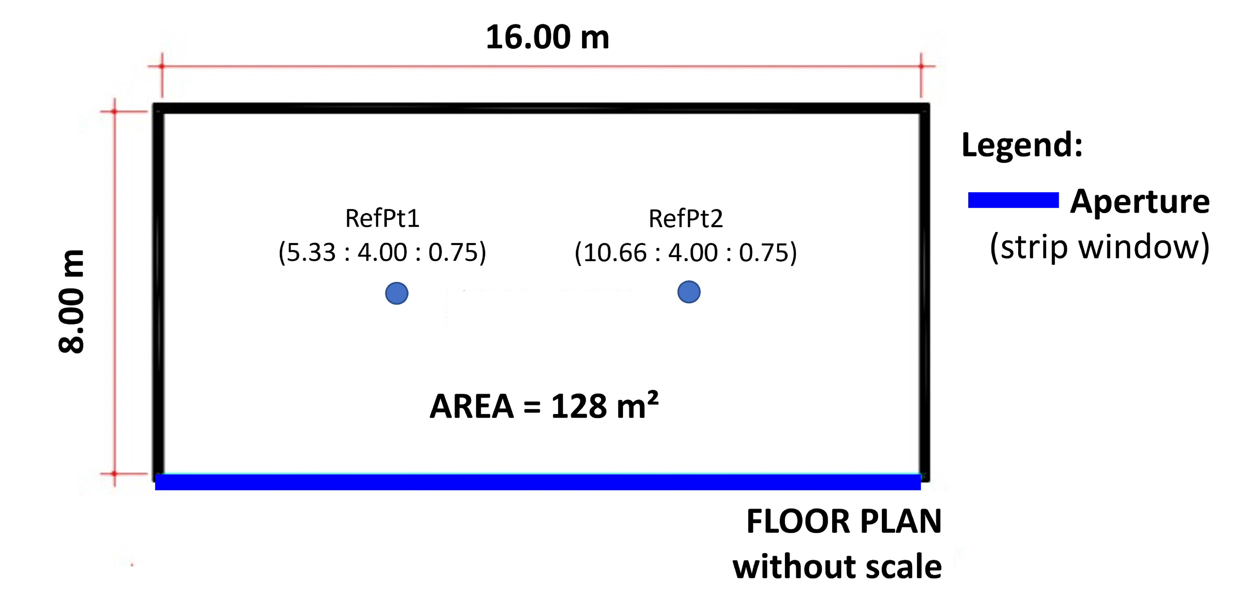
Fig. 3. Floor plan of the hypothetical environment associated with the thermal zone.

The ANNs were trained with data generated by EnergyPlus v. 7.2 [52] thermo-energetic simulations. The performance of the metamodels was assessed by comparing the results predicted by the ANNs with the original thermo-energetic simulation results [53]. Evaluations were carried out with regard to the encoding of the orientation as an input variable of the networks and also to the number of examples required for the learning and the optimization of training parameters. A systematic research study was conducted, progressively, in which the result of each analysis determined the nature of the next one.

3.1. Database: sampling, parameterization and energy simulations

The database presented herein consists of parametric models derived from interactions using only one thermal zone, aiming to compute the effect of orientation (Fig. 3). The parametric combinations included variations in the values for orientation, WWR and VT, as shown in Table 1. The minimum and maximum values for each variable were chosen to avoid the ANN extrapolation, as shown in the following sections. The other values were interpolated aiming at a uniform distribution among the cases of the training set. The sampling was directed, and the values for the key variables were selected according to the investigation stage.

Table 1

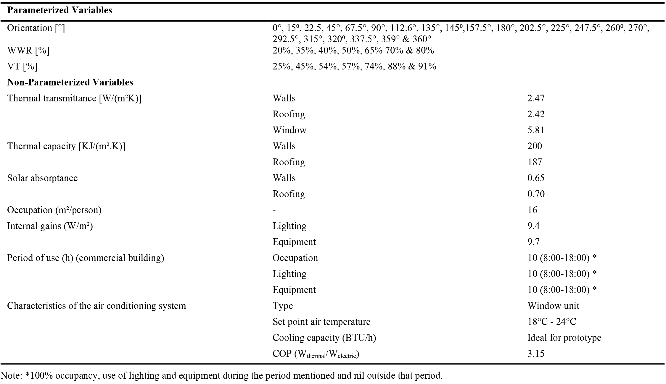
Table 1. Features of the thermal zone.

The thermal zone had a length of 16 m, width of 8 m and floor-to-ceiling height of 3 m, with a strip window along the larger dimension, and is hypothetically located in a commercial building. The space dimensions were defined to minimize an EnergyPlus limitation, which maximizes the effect of daylight reflections in deep rooms [40]. Table 1 shows the thermal properties of the building and the space pattern of use and occupancy, which was not parameterized. The building construction features are representative of the Brazilian building stock [54,55]. The location was fixed (Florianópolis, Santa Catarina State, Brazil) in order to remove the influence of the building location.

It was considered that all the lighting power installed (1203.2 W) was controlled by an ideal linear dimming system that switches the lights off completely when the minimum dimming point is reached. The lighting system is composed only of general lights and the lighting power is equally divided by two daylighting control sensors, located as shown in Fig. 3. The daylighting performance was simulated through the split-flux method (object: Daylighting: Controls / Detailing type: detailed / Lighting control type: Continuous Off). The Daylight reference illuminance was 500 lux.

The model parameterization was carried out using an Excel spreadsheet macro, adapted from Westphal [56], which combines the variables, assembles *.idf files from EnergyPlus, triggers the simulations, and records the results. As an output of the simulations, the energy consumption was obtained for each end use. The results of the simulations were analyzed by orientation aiming to identify possible difficulties posed to the ANN learning process.

3.2. The metamodels

3.2.1. ANN training

The neural networks were generated in two programs: EasyNN-plus [57] and MATLAB [58,59]. EasyNN-plus was used for the network architecture configuration and by default it uses gradient descent. It was chosen because programming is not involved, and it features a tool that indicates the number and the size of the hidden layer [60]. For the analysis of the network optimization we used MATLAB, allowing experimentation with other learning rules, that is, the Levenberg-Marquardt [37] and Bayesian regularization [61].

Multiple training of the same dataset was carried out. In this study, 5 to 10 neural networks were trained for each investigation, allowing us to observe trends in the precision of the network’s predictions. The data was divided into 80% for training and 20% for testing. When applicable, 10-20% of the training dataset was allocated to the validation dataset.

As an activation or transfer function, the linear, the logarithmic-sigmoidal⁶ and the tangent-sigmoidal⁷ functions were tested because of their good applicability [62,45]. The input layer consisted of variations in the three variables investigated: orientation, WWR and VT. The output layer was composed of four building energy performance variables: total energy consumption and consumption for heating, for cooling and for lighting.

The test approach followed the recommendations of Silva [37] to fix the architecture and size of the network and to vary the training set or fix the training set and vary the network architecture. The parameters to control the network training, such as learning, momentum and minimum gradient rates, validation rules and stopping criteria, were defined based on the software default values, data in the literature and experimentation, according to each analysis.

3.2.2. ANN performance analysis

The analysis process was aimed at identifying the simplest feasible network, since the simpler the metamodel the greater its feasibility will be. The tests started from the simplest ANN that could learn and generalize solutions. The simplest ANN structure was defined using the EasyNN software tool, which allows the automatic generation of the smallest network that can learn patterns, according to input data provided by the user [60].

The performance evaluation was based on error analysis, including the mean absolute error (MAE), the mean absolute percentage error (MAPE) and the root mean squared error (RMSE). These errors were evaluated for the training and test sets individually, and for the total dataset. This consideration was made because most of the studies consulted in the literature review presented only the neural network errors for the total dataset. Since the test set is generally smaller than that used for training, the general mean of the network errors tends toward the training error, which, in most cases, is significantly lower than that of the test set, masking the limitations of metamodels.

The consulted literature recommends separating a percentage from the dataset to test the generalization power of the trained network [33]. However, for metamodels based on parametric cases, this method may not be accurate. It is understood that this proposition comes from studies that use real data, such as biological experiments with sample collections in the field. By separating a percentage of the parametric combinations for the test set, the neural network, in a sense, has already "seen" each variable in that form during training, although in a different combination. Aiming at a more rigorous test method, cases were proposed in which none of the values of the input variables had been presented to the network during training, and these are referred to herein as the unseen set of cases.

3.3. Analysis of the orientation input encoding

The network architecture consisted of three nodes in the input layer (orientation, WWR and VT), one hidden layer with six neurons, and four nodes in the output layer (the four energetic performance parameters). The gradient descent algorithm was used, with validation every six cycles and a stopping criterion of an error below 0.001.

For the analysis of the orientation cyclic scale encoding, three alternatives were tested: the azimuthal approach; the cyclical approach; and the azimuthal approach including 359° N.

In the azimuthal approach, the azimuth angle was used as the input code for the networks, considering the four cardinal directions. For the cyclic approach, the encoding corresponded to the absolute value of the difference between the angle itself and a reference angle. The angle of reference adopted was 0° (north). The limitation of this approach is that it does not differentiate between the east and west facades, adopting the same input value for the neural network (90° in both cases). The objective of using the “azimuthal approach including 359° N” was to add information on the scale polarity. The same procedure as the azimuthal approach was adopted, adding cases with the 359° N-oriented facade to the training set.

The parametric models of the training and validation sets consisted of combinations of the four cardinal directions (N, S, E, W); three WWR values (20%, 50% and 80%) and three VT values (25%, 57% and 91%). For the unseen set, the three values of WWR and VT were combined with the azimuths of the intercardinal and secondary intercardinal directions and with the azimuths 15°, 145°, 260° and 320°. In total, 180 parametric models were used.

3.4. Influence of the training sample size for the three input variables

At this stage, the number of examples required for network training for the different key variables was explored. Thus, orientation, WWR and VT were assessed individually. In total, 714 parametric cases were obtained. The same ANN architecture and training configurations described in section 2 were adopted. Three training dataset options were proposed for each of these variables, called Cases A, B and C. Case A was characterized by the smallest training set, which was progressively expanded. The unseen set was kept fixed, allowing a comparison between the performance of the three cases.

For the analysis of the orientation variable, we adopted the azimuthal encoding including 359° N, as described in the previous section. The training set for Case A consisted of the four cardinal orientations and 359° N. Case B included the addition of the intercardinal directions to the Case A training set and for Case C we added the secondary intercardinal directions to the Case B training set (Table 2). The unseen set corresponded to azimuths 15°, 145°, 260° and 320°. All orientation values were combined with the three WWR values and the three VT values used in the previous analysis.

Table 2

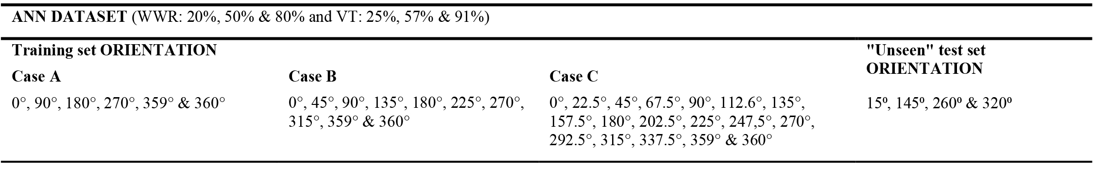
Table 2. Parameterized values for orientation, by analysis group.

For the WWR analysis, Case A consisted of adopting the two extreme values of those used in the previous analysis (20% and 80%), combined with the three values of VT and the five values of orientation, corresponding to the cardinal directions and 359⁰ N (Table 3). In Case B the intermediate value of WWR used in the previous analysis (50%) was added to the Case A training set. For Case C, the intercalated WWR values (35% and 65%) were added to the Case B training set. The additional WWR values in Cases B and C were combined with the same orientation and VT values used in Case A.

Table 3

Table 3. Parameterized values for WWR, by analysis group.

The structuring of the training sets for the VT analysis was similar to that described for the WWR analysis. Therefore, the VT values were added progressively, and combined with the three WWR values and the five orientation values, corresponding to the cardinal directions and 359° N. Table 4 shows the parametric combinations for the three cases of the VT evaluations used for the training set and for the unseen set.

Table 4

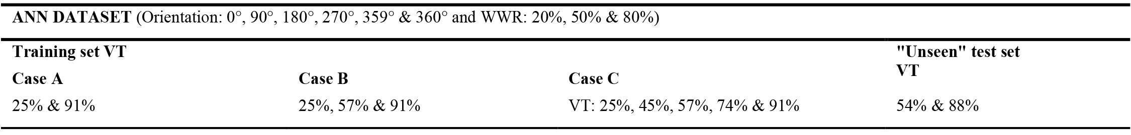
Table 4. Parameterized values for VT, by analysis group.

3.5. Performance analysis of the optimized ANN configuration

Based on the results of the previous stages, the WWR - CASE C training and test sets (Table 3) were adopted to assess the possibility of network optimization by changing its training parameters. Thus, the orientation values corresponded to 0°, 90°, 180°, 270° and 359°, the VT values to 25%, 57% and 91%, and the WWR to 20%, 35%, 50%, 65% and 80%, totalizing 75 training cases.

Regarding the training parameters of the network, an increase to 10 nodes in the hidden layer was tested and also the optimization algorithms Levenberg-Marquardt and Bayesian regularization. The number of neurons determined for the hidden layer size optimization was based on tests reported in the thesis that originated this article [63]. Up to this point, the number of nodes in the hidden layer was 6, indicated by the tool in EasyNN-plus as the simplest network able to learn, and for the gradient descent algorithm the standard of the program was used.

⁶ Logsig: MATLAB sigmoidal logarithmic transfer function. Calculates the value of the output of the neuron from the inputs of the network, that is, the value that will be transferred to the next layer, using a sigmoidal logarithmic function that varies between 0 and +1. It has an "S" format, being a nonlinear function.
⁷ Tansig: MATLAB hyperbolic tangent transfer function. Displays the same definition as the previous function. However, it uses the sigmoidal hyperbolic tangent as a transfer function, which varies between -1 and +1.

4. Results

4.1. Characterization of energy consumption in the databases

The results of the consumption simulations in EnergyPlus were plotted in point (Fig. 4) and bubble (Fig. 5) graphs and presented in distinct scales, due to the difference in the magnitudes of the results. It can be noted that for the total energy consumption (Fig. 4(a)) that the highest amplitude of the results occurs for the northeast and northwest, along with the highest values, since Florianópolis is situated in the southern hemisphere. For the environment typology adopted, the end use with the highest consumption was cooling (Fig. 4(c)), and its distribution was similar to that for the total energy. In the results for the lighting consumption (Fig. 4(d)) the highest amplitude of the results was for the south direction, for which the consumption was higher. The energy consumption associated with heating (Fig. 4(b)) is very low, which may hinder the ANN learning process, since it diverges significantly from the other outputs. These results emphasize the diversity of the responses of the outputs to parametric variations, which indicates that the optimization of networks may require the individualization of outputs for each metamodel.

Figure 4

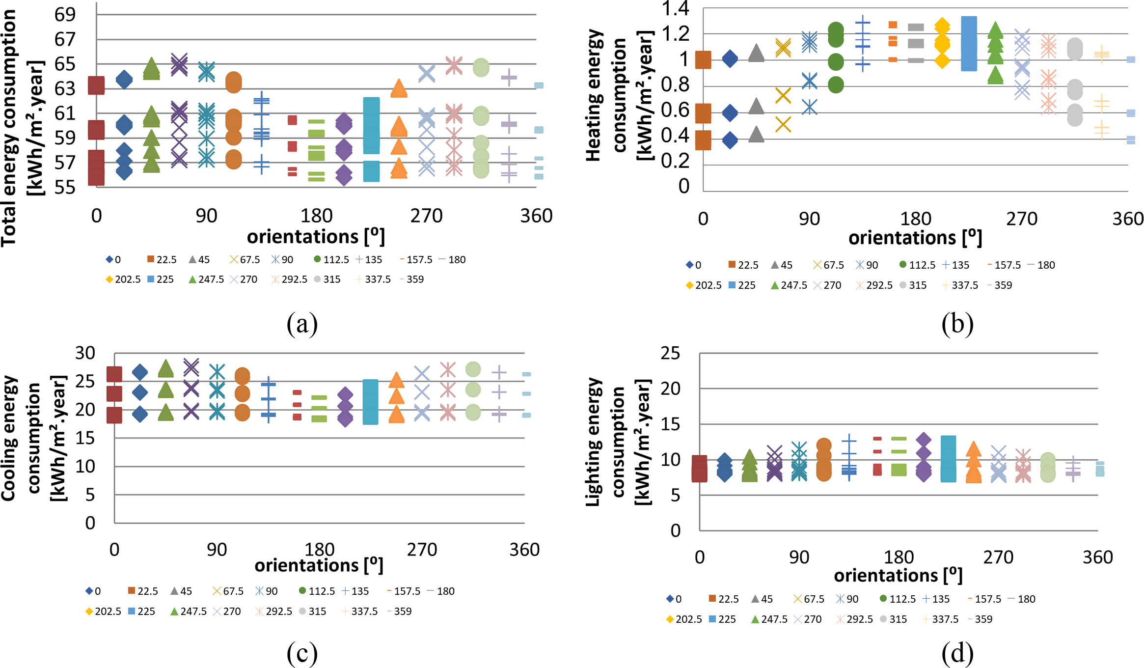
Fig. 4. Energy consumption by orientation and end use.

Figure 5

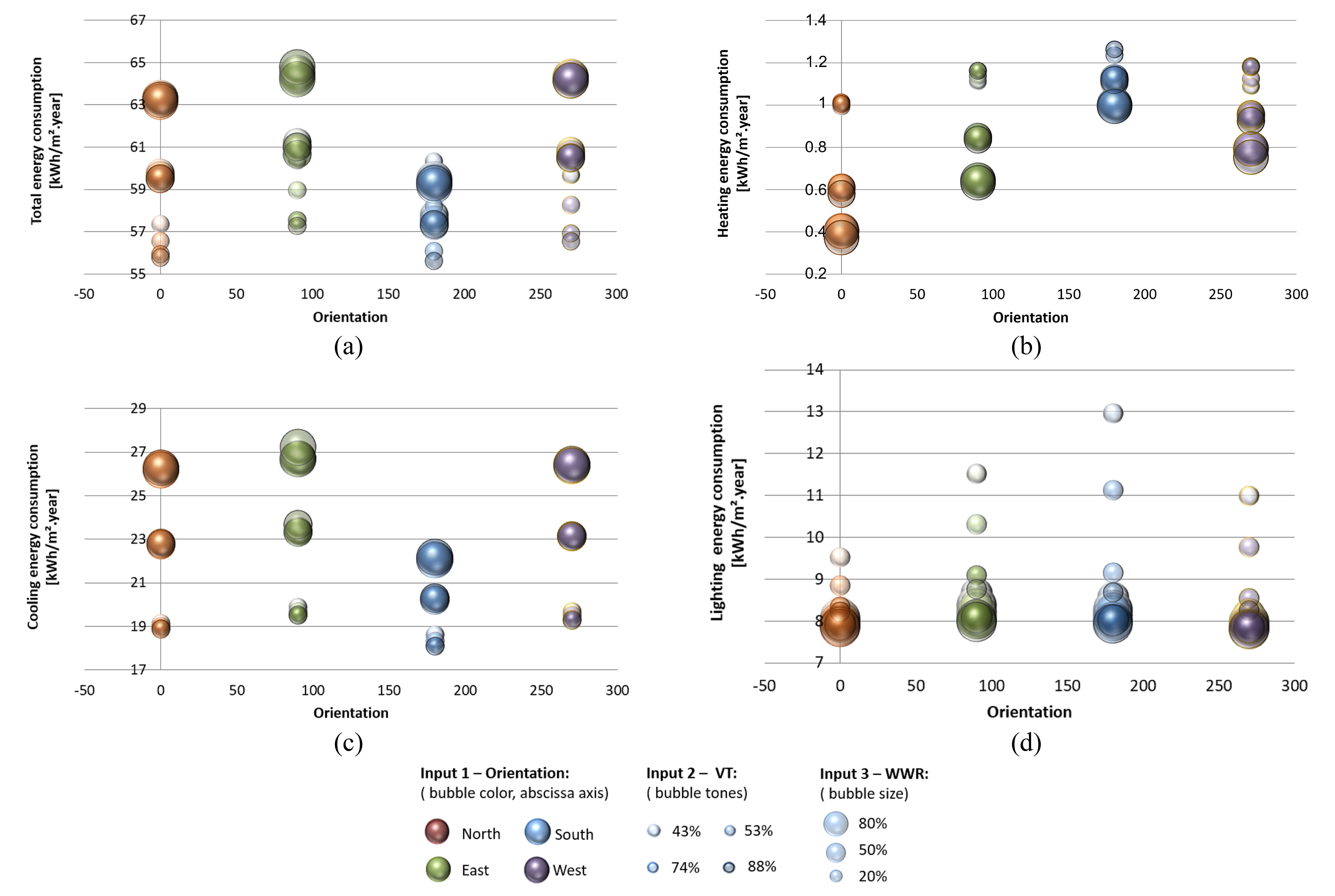
Fig. 5. Energy consumption according to the Orientation, VT and WWR.

The caption for the bubble graph of Fig. 5 adopts the orientation as variable 1 (color, abscissas), VT as variable 2 (color) and WWR as variable 3 (size). In relation to total energy, a challenge identified in the training of the metamodels is the consumption estimation for environments oriented toward the south (Fig. 5(a)) due to the difference in the effects of orientation on the cooling and lighting. In the case of cooling (Fig. 5(c)), this is the orientation that has the data distribution with the lowest amplitude while lighting has the highest amplitude (Fig. 5(d)). The inverse effect that an increase in the WWR has on the consumption associated with cooling and lighting, means that the highest total consumption for this orientation occurs for a small opening with low visible transmission (Fig. 5(a)).

A factor that could hinder the learning of networks as far as cooling consumption is concerned is the effect of daylight harvesting on reducing the thermal load through a reduction in the use of the lighting system and, consequently, the thermal load generated by it. This variation, which would not occur if there was no daylight harvesting, increases the complexity associated with predicting the effect of the combination of WWR and VT, which means that the lowest consumption for WWR 20% would correspond to VT 88% (glass with higher solar factor) and not VT 43%, as it occurred for WWR 50% and 80% (Fig. 5(b)).

4.2. Analysis of the orientation input encoding

To facilitate the analysis, the results were plotted in radial graphs, allowing the observation of the orientations that presented the largest errors. Figure 6 illustrates the MAPE charts for the total energy consumption output parameter, with the errors marked along the radius of the graphs. Each line corresponds to the average MAPE value for the 10 trained ANNs separated by the model characteristics, e.g., the purple line highlighted (red box) in the legend of Fig. 6 represents the average MAPE values for the models with VT 0.57 and WWR 20%, for each orientation. Filled circles correspond to cases in the validation set.

Figure 6

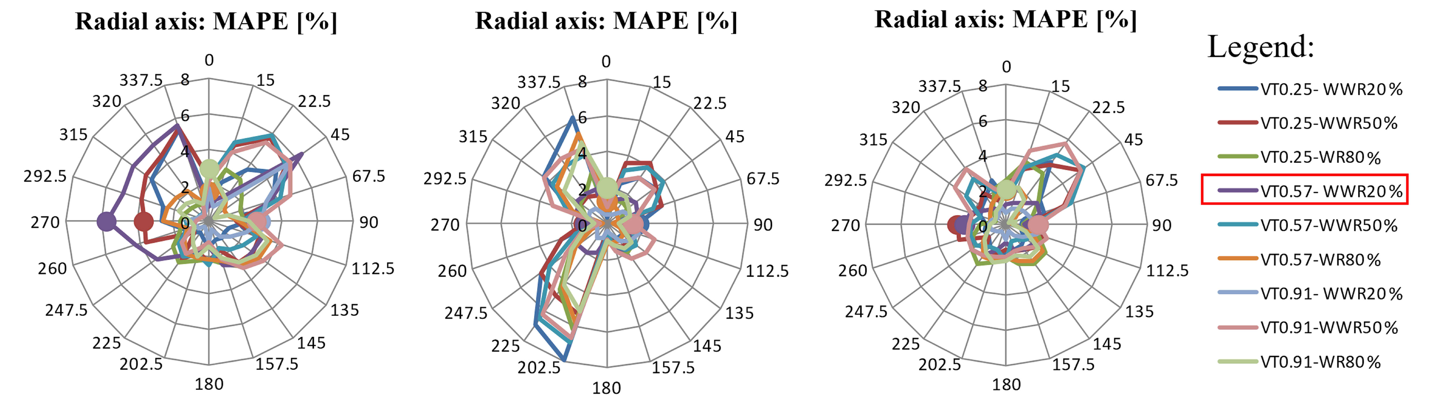
Average MAPE values for the 10 ANNs for each encoding approach: grouped by VT and WWR combination (output parameter: total energy consumption): (a) Azimuthal (b) Cyclic, and (c) Azimuthal + 359° N.

Fig. 6. Average MAPE values for the 10 ANNs for each encoding approach: grouped by VT and WWR combination (output parameter: total energy consumption): (a) Azimuthal (b) Cyclic, and (c) Azimuthal + 359° N.

In general, the errors increased for cyclic encoding in relation to azimuth encoding. The limitations of the cyclic approach, as described in Section 2.3, can be confirmed in the graph of Fig. 6(b), since the networks presented errors of less than 5% for models with the east facing facade and the NE and SE quadrants (right half of the graph), and up to 8% for models oriented to the west and the NW and SW quadrants (left half of the graph). This asymmetry did not occur in either of the other two approaches (the azimuthal and the azimuthal + 359⁰ N). The cases with a west orientation (270°), with errors close to zero, were the cases presented during the training of the networks.

The addition of orientation 359⁰ N to the azimuth approach significantly improved the prediction performance of the networks for the NW quadrant orientations. The average MAPE for all cases in this quadrant was halved, not only for total energy consumption, but also for heating and lighting (Fig. 7). The results showed that the networks were capable of estimating the total consumption for the south facade (Fig. 6(c)) in contrast with the hypothesis suggested in the discussions in the previous section. Although the MAPE of air conditioning consumption for the south surpassed 6% in some cases (Fig. 7(a)), the greatest errors occurred for cases with orientation toward the north quadrants.

Figure 7

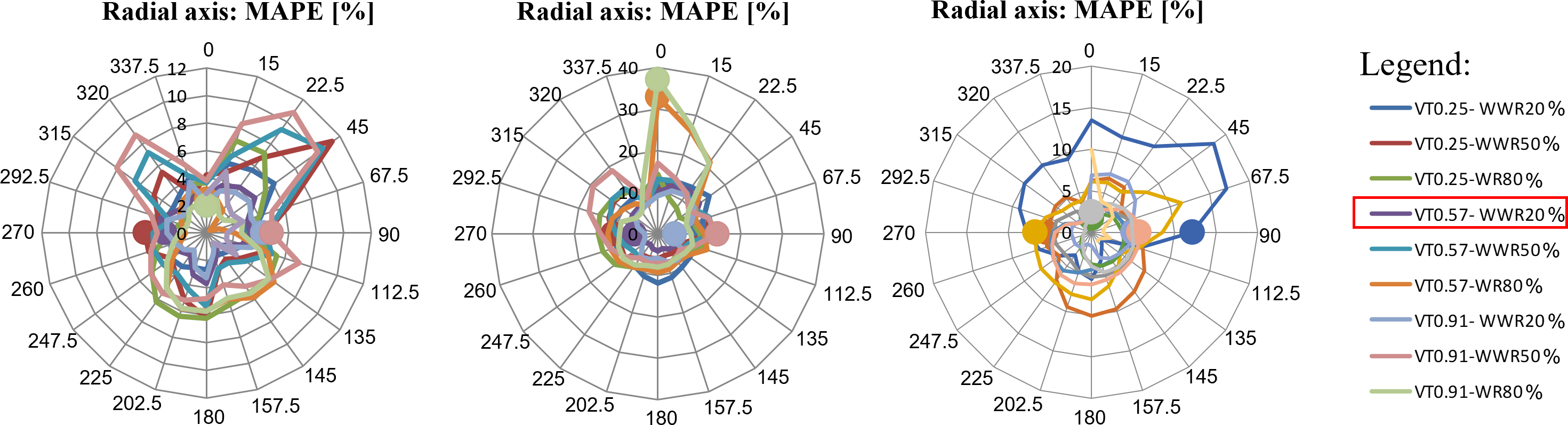
Fig. 7. Average MAPE values for the 10 ANNs for Azimuthal + 359° N: grouped by VT and WWR combination: (a) Cooling (b) Heating and (c) Lighting.

4.3. Analysis of the influence of increasing the examples in the training set

The box plot graphs in Fig. 8 show the results of increasing the number of examples for orientation, WWR and VT. In these graphs, the bars represent the MAPE for each output parameter and the whiskers represent the standard deviation of the set (considering 10 ANNs).

Figure 8

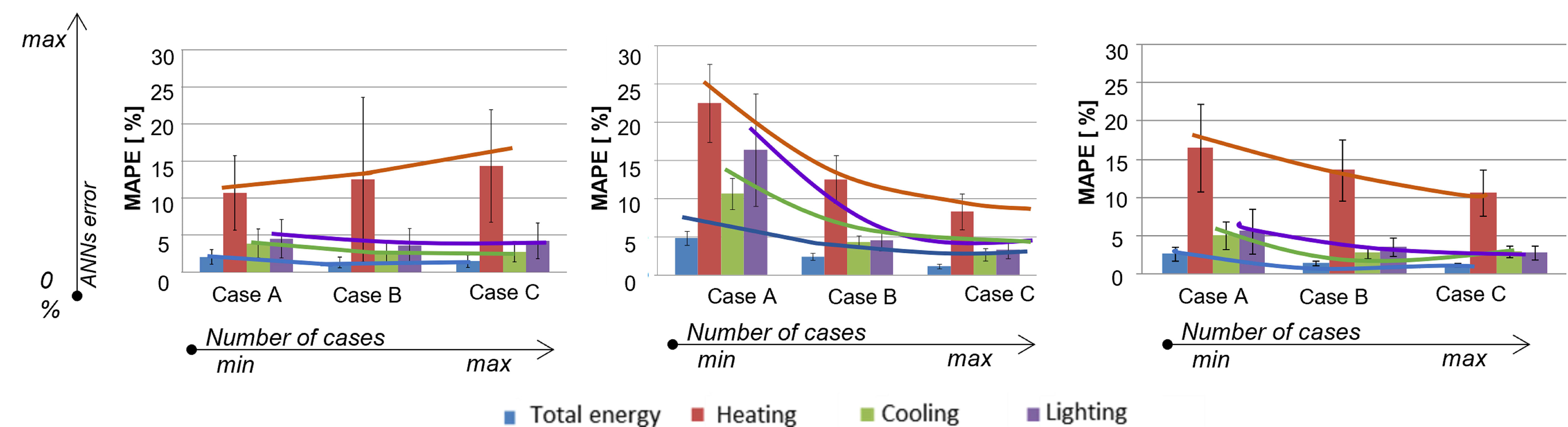
Fig. 8. Trend curves for the network error reduction with an increasing number of training cases - unseen set evaluation: (a) orientation (b) WWR, and (c) VT.

The experiments showed that each input variable has a particular function regarding the relation between the number of examples and the performance of the networks, for each of the 4 output variables. In relation to the 3 input variables studied, orientation and VT resulted in similar functions, but this was not the case for heating. For both orientation and VT, the curves are slightly accentuated. Comparatively, the function representing orientation is less concave compared with VT, due to the greater number of new examples presented to the network in cases B and C, as seen in Figs. 8 (a) and (c). WWR presented a more pronounced parabola with a linear tendency to the right, as seen in Fig. 8(b). VT was the variable that needed fewer examples for the network training. It was observed that for some output variables, an increase in the number of examples can even reduce the performance of the model (e.g., cooling and total energy consumption when the number of VT samples is increased). The curves may change as the variables are combined to produce new parametric models. In this case, new quantities of examples may be required for the network to learn the patterns.

In general, the results in Fig. 8 showed that the networks estimated the total energy consumption with higher precision and the heating energy consumption with lower precision. The existence of four outputs influences the adjustment of the weights of synaptic connections that occur during the network learning process. This interrelation may have benefited the estimate of total energy consumption, which conceptually is the result of the sum of the other output variables. However, it should be noted that for the black box models there is no explicit relation between the physical phenomenon and the model estimate. Although they show a relation, the outputs are, to some extent, independent. Thus, it can not be expected that the errors obtained for the total energy consumption correspond to the average or the sum of the errors for the other variables. The errors are associated with the network power to estimate that output.

The magnitude of the errors obtained for the heating energy consumption, being significantly higher than those of the other outputs, is due to the absolute values employed to train the networks. These values were extremely low due to the Brazilian climatic conditions, lower than 1.4 kWh/m2/year. On the other hand, the consumption values were limited to 69 kWh/m2/year for total energy, to 25 kWh/m2/year for cooling and to 20 kWh/m2/year for lighting. Therefore, even though the percentage errors are much higher in relation to the other variables, they are insignificant in terms of absolute consumption.

It can be observed in Fig. 8(a) that the errors for the heating energy consumption show a progressive increase from Case A to Case C. This variation was not considered representative, since the values obtained for the heating consumption were practically null. Furthermore, the difference between the magnitudes of the consumption of the output variables may hinder the learning of the networks and also may explain the divergences between the error patterns of the four output variables.

Regarding the orientation variable, an increase in the number of examples did not improve the network performance to the point of justifying the increased computational effort required for the energy simulations. When evaluating the effects of including the new examples for each output variable separately, the most significant error reductions occurred for cooling and lighting, from 3.3% to 2.9% and from 4.7% to 4.2%, respectively. These variations were observed in the errors for cases oriented to the northern quadrants (NE and NW) and correspond to the mean MAPE of the 10 trained ANNs. When evaluated individually, it was possible to observe that the improvement in the network performance was due to a reduction in the errors associated with the outliers.

Overall errors were also verified considering the mean of all output variables, for the training and test sets. An increase in the number of samples for the orientation worsened the training set performance, increasing the overall MAPE from 4.8% for Case A, to 5.16% for Case B and 5.36% for Case C. On the other hand, for the unseen set, the overall MAPE decreased from 5.27% for Case A to 5.03% for Case B and increased to 5.69% for the Case C orientations.

Increasing the number of WWR examples also led to different results for the training set and for the unseen set. For the training set, Case A presented the smallest errors for the 4 output parameters, followed by Case C and then Case B. For the unseen set (Fig. 8(b)), adding new examples from Case A to Case B and Case C improved the network performance for the 4 output parameters progressively.

Likewise, an increase in the number of VT samples led to different results for the training set and for the unseen set. In general, training set errors varied very little on including new examples, less than 1% in absolute terms. Even so, the smallest errors corresponded to Case A. For the unseen set (Fig. 8(c)), in contrast to the WWR results, there was no uniform pattern in the response to the increase in samples for all output parameters. For cooling, the performance improved from Case A to Case B, but worsened from Case B to Case C. Total energy consumption, heating and lighting presented reductions in the errors from Case A to Case B and from Case B to Case C.

With regard to the individual evaluation of the 10 ANNs, a large variability in the performance of the different networks was observed for the three experiments (considering the orientation, WWR and VT). However, it can be observed that this variability is lower when one of the input variables outperforms the other. In this case, the disturbance of the least impacting variable does not cause significant changes in the output variables. To exemplify this finding, Fig. 9 illustrates the MAPE for each of the 10 ANNs considering the VT investigation examples. Here, the networks were trained with the Case A set (see Table 4), for the total energy consumption output parameter, considering only the cases oriented to the north, grouped according to the three WWR values. When the WWR is expressive (80%), the VT variation has a lower impact on consumption and therefore the results estimated by the networks presented a more constant error pattern (Fig. 9(c)). This trend in the behavior was repeated for the other three orientations evaluated.

Figure 9

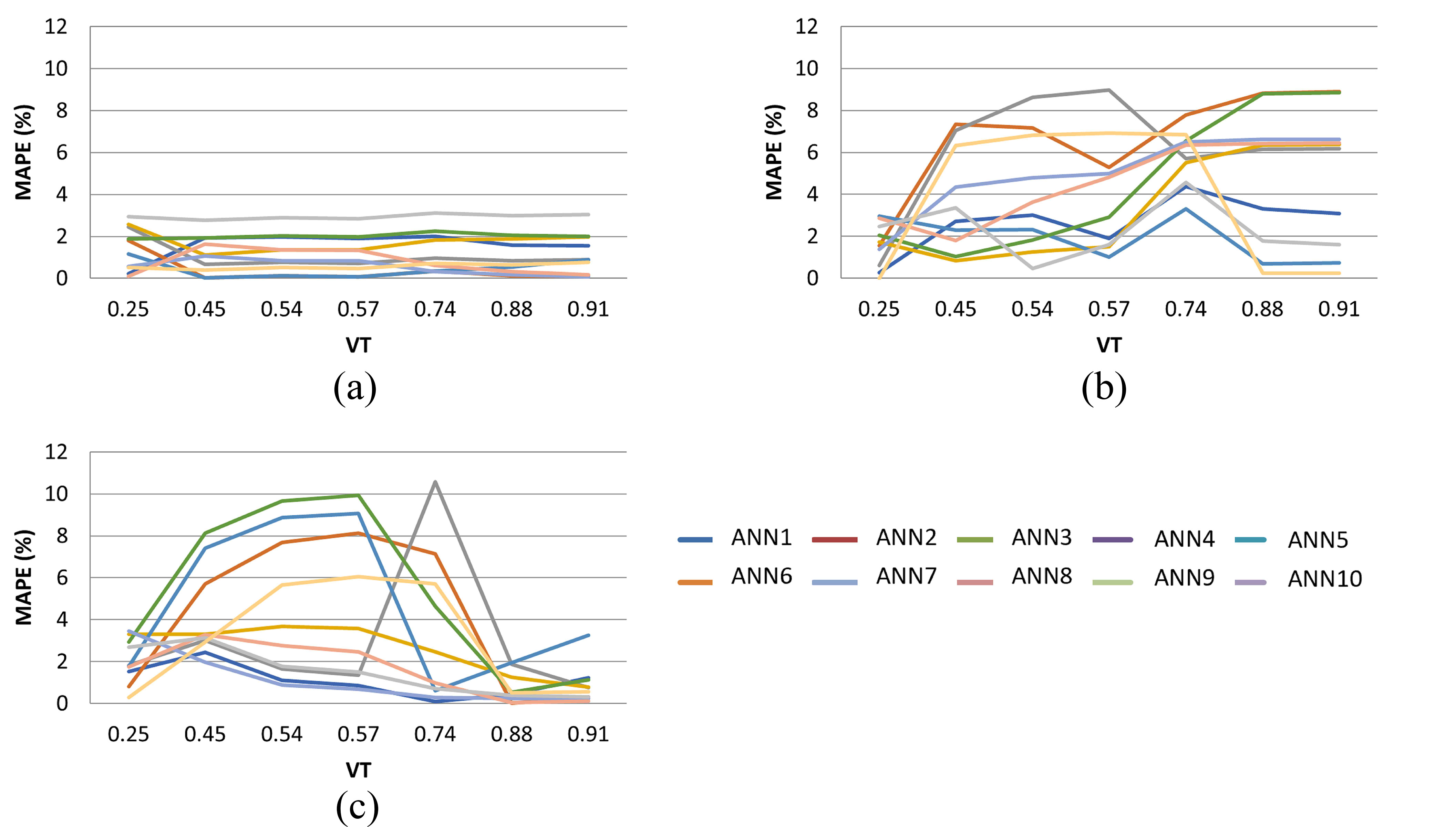
Performance of the 10 ANNs for the total dataset of Case A - VT (north orientation, output parameter: total energy consumption): (a) WWR 20% (b) WWR 50%, and (c) WWR 80%.

Fig. 9. Performance of the 10 ANNs for the total dataset of Case A - VT (north orientation, output parameter: total energy consumption): (a) WWR 20% (b) WWR 50%, and (c) WWR 80%.

4.4. Optimized configuration for the ANNs

Increasing the number of neurons significantly improved the performance of the network for all of the output parameters. The series of blue bars in Figs. 10(a) and (b) corresponds to the same network shown for Case C in Fig. 8(b), the network with 6 nodes in the hidden layer employing the gradient descent algorithm. The series of red bars in Figs. 10(a) and (b) shows the results for the network of the same algorithm, however with 10 neurons in the hidden layer.

Figure 10

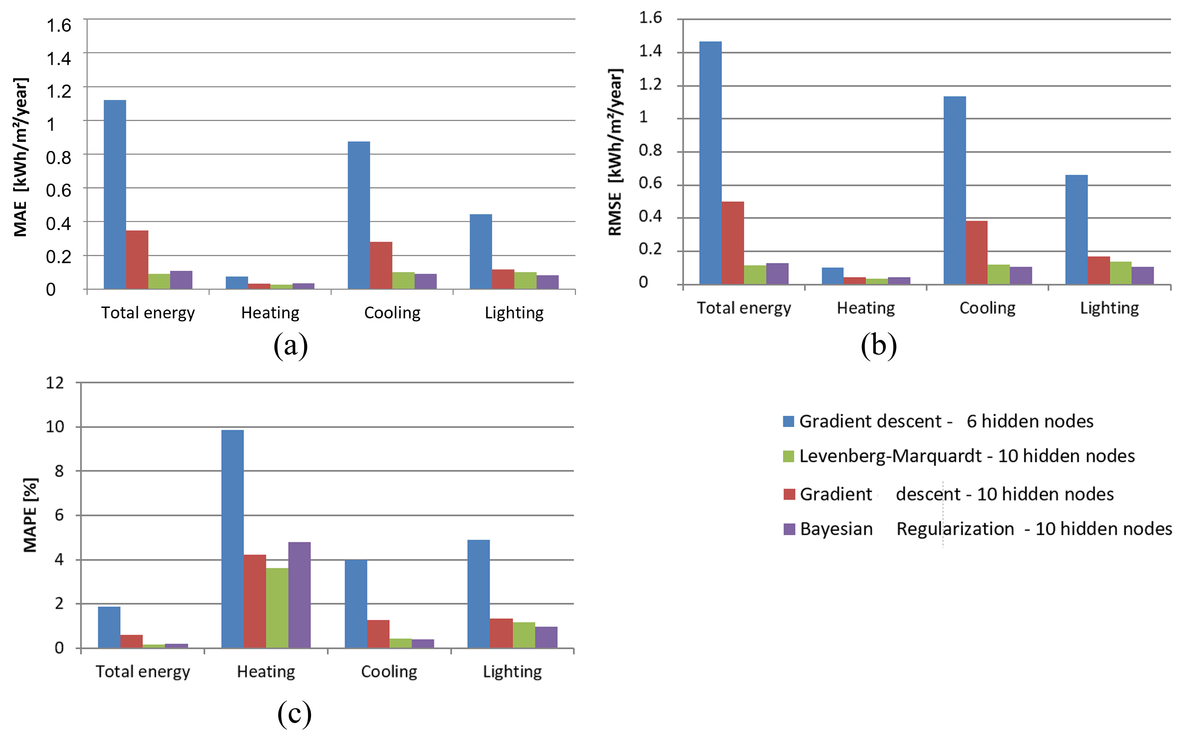
Fig. 10. Performance of optimized ANNs by output – unseen set: (a) MAE (b) RMSE, and (c) MAPE.

The performance of the Levenberg-Marquardt and Bayesian regularization algorithms was slightly higher than that of the gradient descent algorithm. The Bayesian regularization showed smaller errors than the Levenberg-Marquardt algorithm for the cooling and lighting and greater errors for the total consumption and heating. Although the difference between the algorithms in terms of performance was small, the processing speed varied considerably. The processing for the two aforementioned algorithms was more rapid (less than 10 min) compared with the gradient descent algorithm (1.0-2.5 h). The balance between performance and processing speed led to the adoption of the Bayesian regularization algorithm being considered most advantageous for this metamodel.

5. Discussion

In this initial stage of the construction of the simplified tool, aspects related to the modeling of the building's orientation and the configuration of the ANN were approached, including the definition of the training set. The investigation reported herein demonstrates the relevance of the parameters of network training and the difficulty associated with establishing a set of examples for the training of a black box model, since an increase in the number of examples does not necessarily reflect in its optimization. In architecture, the design possibilities are endless and, although technology allows the simulation of large sets of data, limitations are inevitable. A notable contribution of this study is that it provides an indication of how to approach the variable orientation as an input parameter of the metamodel.

The hypotheses raised by the analysis of the simulated database were not confirmed. The greatest errors were associated with the orientations which receive more solar radiation, that is, the north quadrants rather than the south quadrants, as expected. This leads to the conclusion that for these networks, which are black box models, when there is daylight harvesting the effect of the relation between WWR and VT on the energy consumption does not hinder the modeling (whereas it could for white and gray box models).

The results of this study indicate that ANNs have the potential to predict consumption when there is daylight harvesting, however, this is based on a restricted range of architectonic variations focused on the building envelope. The next steps for the development of the simplified tool should address larger parametric sets, which incorporate other key variables of the building described. The first expansion of the metamodel should address the exploration of environments with other geometries, since the effect of WWR on energy consumption may differ greatly for environments with the same floor area, varying only the proportion between width and depth, as shown by the comparison in Fig. 11. It can be noted that the complexity of the problem increases when the geometry in relation to the orientation is added as a variable. Both models have the same area, volume and lighting plan and were compared considering the same WWR values. The difference in the profiles of the curves for total consumption, heating, cooling and lighting presents a potential challenge in dealing with different geometries with different orientations in modelling with ANNs.

Figure 11

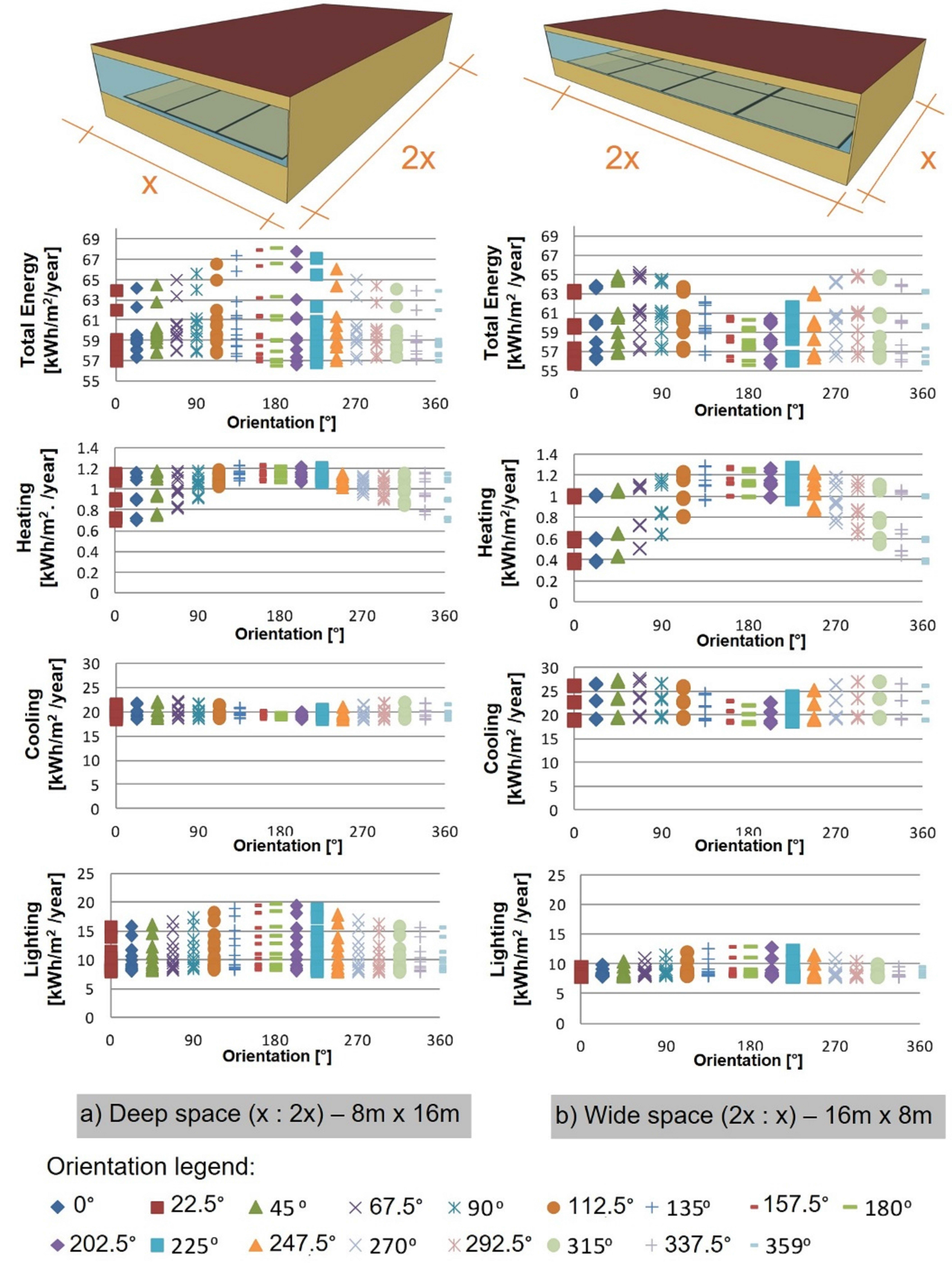
Fig. 11. Energy consumption of two geometries: deep and wide, for the 17 orientations.

The sequence of the expansion of the metamodel scope will involve the incorporation of other façade elements and the architectural configuration of the environments, followed by elements that describe the context of the building's insertion, such as obstructions caused by the surroundings and the geographic location. In these stages, a migration from the EnergyPlus program to others based on Radiance is foreseen. EnergyPlus was adopted in the initial stages of the development of the tool to allow greater agility in the generation of the database and to investigate the details of the application of ANNs to this process. However, once the details of the network configuration have been selected, physical complexities will be incorporated into the model, requiring more accurate daylighting simulation programs.

It should be noted that the results obtained so far do not apply only in the context of the construction of the simplified tool that motivated this study, but to other similar applications where ANNs are used. Although the simulations were generated in the EnergyPlus program by the split-flux method, the choice of a simple geometry that minimizes its limitations allows the results obtained on the network metamodeling potential to be extended to other simulation methods.

6. Conclusions

The results obtained in the first stage of the development of a simplified tool for estimating the impact of daylight harvesting on the energy consumption of buildings are reported in this paper. The potential of ANNs to model the effect of orientation and important aspects of their configuration were investigated. The results reported herein contribute to improving our understanding of how ANNs, as black box models, respond to the effect of orientation on the energy consumption when there is daylight harvesting. Feed forward networks with supervised learning, and the use of the error backpropagation algorithm, were the subject of this study. The networks were analyzed considering the elementary variables of the building envelope: orientation, WWR and VT. It is shown that the networks estimated the individualized consumption by orientation with errors below 5% for new cases. The analysis of the input variables revealed that the encoding on a cyclical scale of the orientation must indicate its beginning and end. It also showed that the 3 variables require different amounts of examples for the network training and highlighted the relevance of the architectural configurations and the training of the networks with regard to their performance. These results suggest that the ANNs are potential techniques for application in the development of simplified tools, in order to aid the designer and maximize the daylight harvesting, considering the particularities of each orientation. The evidence regarding the precision of consumption estimates obtained considering elementary variables of the building envelope, the characterization of the scale associated with the orientation and the singular approach to the variables, contribute as guidelines for the production of new metamodels with a broader scope.

Acknowledgment

This study was financed by CAPES - Brazil - Finance Code 001 and by CNPq - Brazil - Finance Code 151162/2019-0 and 307179/2016-8.

R. W. da Fonseca would like to thank Prof. Mauro Roisenberg and Dr. Isaac Sacramento for the valuable support regarding the application of artificial intelligence. Also, Prof. Fernando S. Westphal kindly provided the base of the Excel macro, used for the parameterization of the models and the energy simulations. Finally, the authors are grateful to Prof. Konstatinos Papamichal for the in-depth discussions on the development of tools for estimating the potential of daylight harvesting for energy savings.

Contributions

R. W. da Fonseca: Conceptualization, Methodology, Formal analysis, Investigation, Writing - Original Draft. F. O. R. Pereira: Reviewing and Supervision.

Declaration of competing interest

The authors declares that there is no conflict of interest.

References

L. Heschong, Daylight Metrics. Heschong Mahone Group - Public Interest Energy Research - California Energy Commission, Feb. 2012. (CEC-500-2012-053),pp. 387.
C. Gehbauer, D.H. Blum, T. Wang, E.S. Lee, An assessment of the load modifying potential of model predictive controlled dynamic facades within the California context, Energy Build. 210 (2020) 1-24. https://doi.org/10.1016/j.enbuild.2020.109762
M. Kenney, H. Bird, H. Rosales, 2019 California Energy Efficiency Action Plan. California Energy Commission, 2019. 110 p. (CEC400-2019-010-SF).
A. Williams, et al., Lighting Controls in Commercial Buildings. LEUKOS - Journal of Illuminating Engineering Society of North America 8: 3 (2012) 161-180. https://doi.org/10.1582/leukos.2012.08.03.001
C. S. Jardim, et al., The potential of grid-connected photovoltaic systems in urban areas: two case studies, in: Proceedings…5th Enc. Energ. Meio Rural, 2004, pp. 1 – 12, Campinas, Brazil (in Portuguese).
F. O. R. Pereira, et al., An investigation about the consideration of daylighting along the design stages, in: Proceedings... Passive and Low Energy Architecture, 2005. pp. 1025-1030, Beirut.
F. O. R. Pereira, Luminous and thermal performance of shading and sunlighting reflecting devices. (PhD thesis) Building Science Unit School of Architectural Studies University of Sheffield, University of Sheffield, Sheffield, 1992, pp. 301.
D. B. Crawley, W. J. Hand, M. Kummert, B. T. Griffith, Contrasting the capabilities of building energy performance simulation programs, Washington, DC: US Department of Energy, 2005. https://doi.org/10.1016/j.buildenv.2006.10.027
S. Kota, J. S. Haberl, Historical survey of daylighting calculations methods and their use in energy performance simulations, in: Proceedings of International Conference for Enhanced Building Operations, 2009, 1-9, Austin.
CSBR, LBNL, Façade Design Tool, Minneapolis. 2012. Available from: < http://www.commercialwindows.org/fdt.php >. Accessed: Mar. 2014.
T. R. C. - H. M. G, SkyCalcTM. 3.0 Energy Design Resources, 2009.
T. R. C. - H. M. G, Skylighting Design Guidelines: energy design resources, California Public Utilities Commission, 2014. pp. 133.
T. A. Gibson, Daylighting software validation study and development of a simplified method to predict the energy impacts of facade design and daylighting control in private offices, ProQuest Diss Theses [Internet], 2011, pp. 273.
D. H. W. Li, S. L. Wong, K. L. Cheung, Energy performance regression models for office buildings with daylighting controls, in: Proceedings... Institution of Mechanical Engineers, Part A: Journal of Power and Energy: SAGE, 2008, pp. 557-568. https://doi.org/10.1243/09576509jpe620
S. Moret, M. Noro, K. Papamichael, Daylight harvesting: a multivariate regression linear model for predicting the impact on lighting, cooling and heating, in: Proceedings... Building Simulation Applications BSA 2013, 2013, pp. 39 – 48, Bolzano.
E. L. Didoné, F. O. R. Pereira, Integrated computational simulation for the consideration of daylight in the energy performance evaluation of buildings, Ambient. constr. 10 (2010) 139-154.
C. Qiu, et al., Coupling an artificial neuron network daylighting model and building energy simulation for vacuum photovoltaic glazing, Applied Energy 263 (2020) 1-15. https://doi.org/10.1016/j.apenergy.2020.114624
K. LI, et al., Forecasting building energy consumption using neural networks and hybrid neuro-fuzzy system: A comparative study, Energy and Buildings 43 (2011) 2893-2899. https://doi.org/10.1016/j.enbuild.2011.07.010
A. H. Neto, F. A. S. Fiorelli, Comparison between detailed model simulation and artificial neural network for forecasting building energy consumption, Energy and Buildings 40 (2008) 2169-2176.
M. S. Mayhoub, D. J. Carter, Towards hybrid lighting systems: A review, Lighting Research & Technology 42 (2010) 51-71. https://doi.org/10.1177/1477153509103724
M. Krarti, An Overview of Artificial Intelligence-Based Methods for Building Energy Systems, Journal of Solar Energy Engineering 125: 3 (2003) 331-342. https://doi.org/10.1115/1.1592186
D. Coakley, et al., A review of methods to match building energy simulation models to measured data, Renewable and Sustainable Energy Reviews 37 (2014) 123-141. https://doi.org/10.1016/j.rser.2014.05.007
N. Fumo, A review on the basics of building energy estimation. Renewable and Sustainable Energy Reviews 31 (2014) 53-60. https://doi.org/10.1016/j.rser.2013.11.040
N. D. Roman, et al., Application and characterization of metamodels based on artificial neural networks for building performance simulation: a systematic review, Energy and Buildings 217 (2020) 1-22. https://doi.org/10.1016/j.enbuild.2020.109972
S. L. Wong, et al., Artificial neural networks for energy analysis of office buildings with daylighting, Applied Energy 87 (2010) 551-557. https://doi.org/10.1016/j.apenergy.2009.06.028
R. W. Fonseca, E. L. Didoné, F. O. R. Pereira, Using artificial neural networks to predict the impact of daylighting on building final electric energy requirements, Energy and Building 61 (2013) 31-38. https://doi.org/10.1016/j.enbuild.2013.02.009
W. Kim, Y. Jeon, Y. Kim, Simulation-based Optimization of an Integrated Daylighting and HVAC System Using the Design of Experiments Method, Applied Energy 162 (2016) 666–674. https://doi.org/10.1016/j.apenergy.2015.10.153
J. Hu, S. Olbina, Illuminance-based slat angle selection model for automated control of split blinds. Building and Environment 46: 3 (2011) 786-796. https://doi.org/10.1016/j.buildenv.2010.10.013
N. V. Katsanou, et al., An ANN-based model for the prediction of internal lighting conditions and user actions in non-residential buildings, Journal of Building Performance Simulation 120 (2019) p. 125-132. https://doi.org/10.1080/19401493.2019.1610067
C. L. Lorenz, et al., Artificial Neural Networks for parametric daylight design, Architectural Science Review 63:2 (2019) 210-221. https://doi.org/10.1080/00038628.2019.1700901
B. B. Ekici, U. T. Aksoy, Prediction of building energy consumption by using artificial neural networks. Advances in Engineering Software 40: 5 (2009) 356-362. https://doi.org/10.1016/j.advengsoft.2008.05.003
A. P. Melo, et al. Development of surrogate models using artificial neural network for building shell energy labeling, Energy Policy 69 (2014) 1-9. https://doi.org/10.1016/j.enpol.2014.02.001
S. Haykin, Artificial Neural Networks: Principles and Practices, second ed., Bookman, Porto Alegre, 900 p. (in Portuguese). 2001.
Y. Zhang, et al., Comparisons of inverse modeling approaches for predicting building energy performance, Building and Environment 86 (2015) 177-190. https://doi.org/10.1016/j.buildenv.2014.12.023
T. Kazanasmaz, M. Günaydin, S. Binol, Artificial neural networks to predict daylight illuminance in office buildings, Building an Environment 44 (2009) 1751-1757. https://doi.org/10.1016/j.buildenv.2008.11.012
R. A. Kilmer, Artificial Neural Network Metamodels of Stochastic Computer Simulations, (PhD Thesis) Engineering School, University of Pittsburgh, Pittsburgh, 1994, pp. 234.
R. M. Silva, Artificial Neural Networks applied to Intrusion Detection in TCP / IP Networks, (Master Thesis) Pontifical Catholic University of Rio de Janeiro, Rio de Janeiro, 2005, pp. 144 (in Portuguese). https://doi.org/10.18057/icass2018.p.116
R. W. Fonseca, F. O. R. Pereira, K. Papamichael, The potential of artificial neural networks to model daylight harvesting in buildings located in different climate zones, in: Proceedings... 15th IBPSA Conference, 2017, pp. 1-10, San Francisco, CA, USA. https://doi.org/10.26868/25222708.2017.570
H. Shen, T. Zempelikos, Sensitivity analysis on daylighting and energy performance of perimeter offices with automated shading, Building and Environment 59 (2013) 303-314. https://doi.org/10.1016/j.buildenv.2012.08.028
R. Blanning, The Construction and Implementation of Metamodels, Simulation 24 (1975) 177-184. https://doi.org/10.1177/003754977502400606
W. S. Meisel, D. C. Collins, Repro-Modeling: An Approach to Efficient Model Utilization and Interpretation, IEEE Systems, Man and Cybernetics Society 3 (1973) 349-358. https://doi.org/10.1109/tsmc.1973.4309245
G. C. F. Costa, An energy consumption evaluation conserning transport in the state of Sao Paulo cities, (Master Thesis) Department of Civil Engineering, University of Sao Paulo, Sao Carlos, 2001, pp. 103. https://doi.org/10.21475/ajcs.18.12.07.pne1013
A. R. M. Silva, et al., Performance analysis of artificial neural networks for automatic classification of web spam, Brazilian Journal of Applied Computing 4: 2 (2012) 42-57 (In Portuguese).
H. Liu. On the Levenberg-Marquardt training method for feed-forward neural networks, in: Proceedings of International Conference on Natural Computation, 2010, pp. 456-460. https://doi.org/10.1109/icnc.2010.5583151
The Mathworks Inc., MATLAB Documentation, Natick: The MathWorks Inc, 2014.
K. Madsen, H. B. Nielsen, O. Tingleff, Methods for non-linear least squares problems, second ed., Informatics and Mathematical Modelling, Technical University of Denmark, 2004, pp. 58.
D. D. Ferreira, et al., Automatic system for detection and classification of electrical disturbances in electrical energy quality, Sba Controle & Automação 20: 1 (2009) (In Portuguese).
D. J. C. Mackay, Bayesian Interpolation, Neural Computation 4: 3 (1992) 415-447. https://doi.org/10.1162/neco.1992.4.3.415
T. B. Rodrigues, J. L. R. Macrini, E. C. Monteiro, Selection of variables and classification of patterns by neural networks as an aid to the diagnosis of ischemic heart disease, Pesqui. Oper. 28: 2 (2008) 285-302. https://doi.org/10.1590/S0101-74382008000200007
V. H. Ferreira, Neural models regularization techniques applied to short-term load forecasting, (Master Thesis) Department of Civil Engineering, Federal University of Rio de Janeiro – COPPE, 2005, 204 p. (in Portuguese).
G. Yahiaoui, P. Da Silva Dias, NEXYAD: What is a mathematical model? © NEXYAD Available from: < http://www.nexyad.net/HTML/e-book-Matematical-Model.html >. Accessed in: Sept. 2014.
D.O.E - US. Department of Energy, Energy Plus program. v.6. Available from: < https://energyplus.net/ >. Accessed in: Oct. 2012.
F. C. Winkelmann, S. Selkowitz, Daylighting simulation in the DOE-2 building energy analysis program, Energy and Buildings 8 (1985) 271-286. https://doi.org/10.1016/0378-7788(85)90033-7
M. V. Santana, Influence of construction parameters for energy consumption in office buildings located in Florianopolis-SC, (Master Thesis) Department of Civil Engineering, Federal University of Santa Catarina, 2006, 181 p. (in Portuguese).
J. C. Carlo, Development of methodology for evaluating the envelop energy efficiency of non-residential buildings, (PhD Thesis) Department of Civil Engineering, Federal University of Santa Catarina, 2008, 196 p. (in Portuguese).
F. S. Westphal, Macro Excel Visual Basic for Energy Plus *.idf file parameterization, 2012.
S. Wolstenholme, EasyNNplus software v.1.6, 2013.
The Mathworks Inc., MATLAB - Technical computational language, Natick, 2011.
The Mathworks Inc., MATLAB - Neural Network Toolbox, Natick, 2011.
S. Wolstenholme, EasyNNplus: user interface manual, 2013.
D. J. C. Mackay, Bayesian Interpolation, Neural Comput. 4: 3 (1992) 415–447. https://doi.org/10.1162/neco.1992.4.3.415
W. Duch, N. Jankowski, New neural transfer functions, International Journal of Applied Mathematics and Computer Science 7 (1997) 639 -658.
R. W. Fonseca, Daylighting harvesting for non-residential buildings: the possibilities and limitations of the artificial neural networks, (PhD Thesis) Department of Civil Engineering, Federal University of Santa Catarina, 2015, 457 p. (In Portuguese).

Get PDF (9.45 MB)

SHARE ON