Design and Simulation of a Circadian Lighting Control System Using Fuzzy Logic Controller for LED Lighting Technology

Sivachandran R. Perumal; Faizal Baharum

doi:10.15627/jd.2022.5

Article Outline

3. Results and analysis

Declaration of competing interest

References

Figures and tables

Figures (30)

Tables (11)

Volume 9 Issue 1 pp. 64-82 • doi: 10.15627/jd.2022.5

Design and Simulation of a Circadian Lighting Control System Using Fuzzy Logic Controller for LED Lighting Technology

Sivachandran R. Perumal,^* Faizal Baharum

Author affiliations

School of Housing, Building & Planning, Universiti Sains Malaysia, 11800 Pulau Pinang, Malaysia

*Corresponding author.
siva_rocks@yahoo.com (S. R. Perumal)
baharumfaizal@gmail.com (F. Baharum)

History: Received 26 September 2021 | Revised 24 April 2022 | Accepted 26 April 2022 | Published online 26 May 2022

Citation: Sivachandran R. Perumal, Faizal Baharum, Design and Simulation of a Circadian Lighting Control System Using Fuzzy Logic Controller for LED Lighting Technology, Journal of Daylighting 9 (2022) 64-82. https://dx.doi.org/10.15627/jd.2022.5

Figures and tables

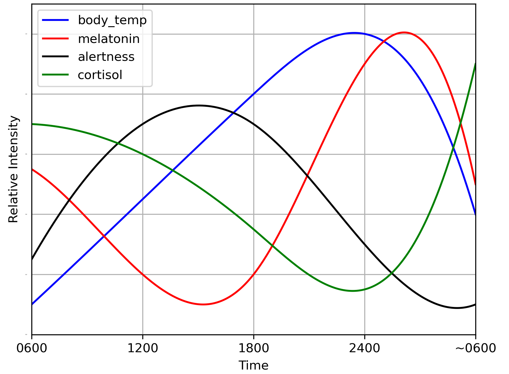Figure 1
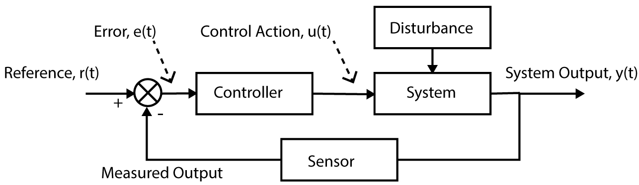Figure 2
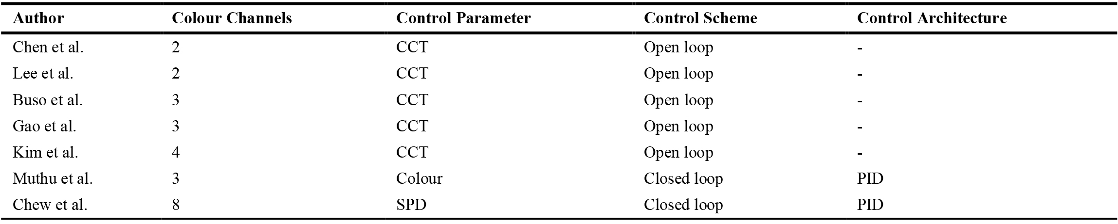Table 1
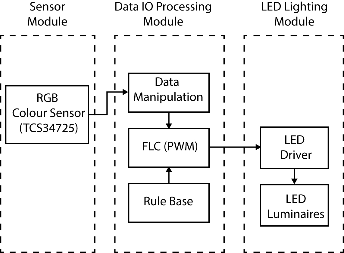Figure 3
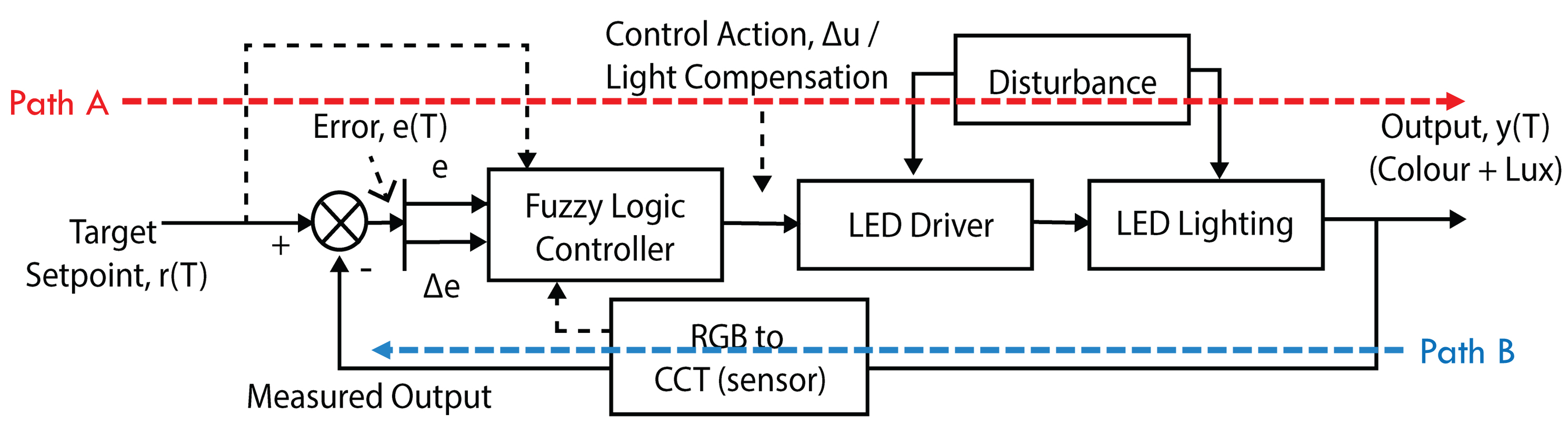Figure 4
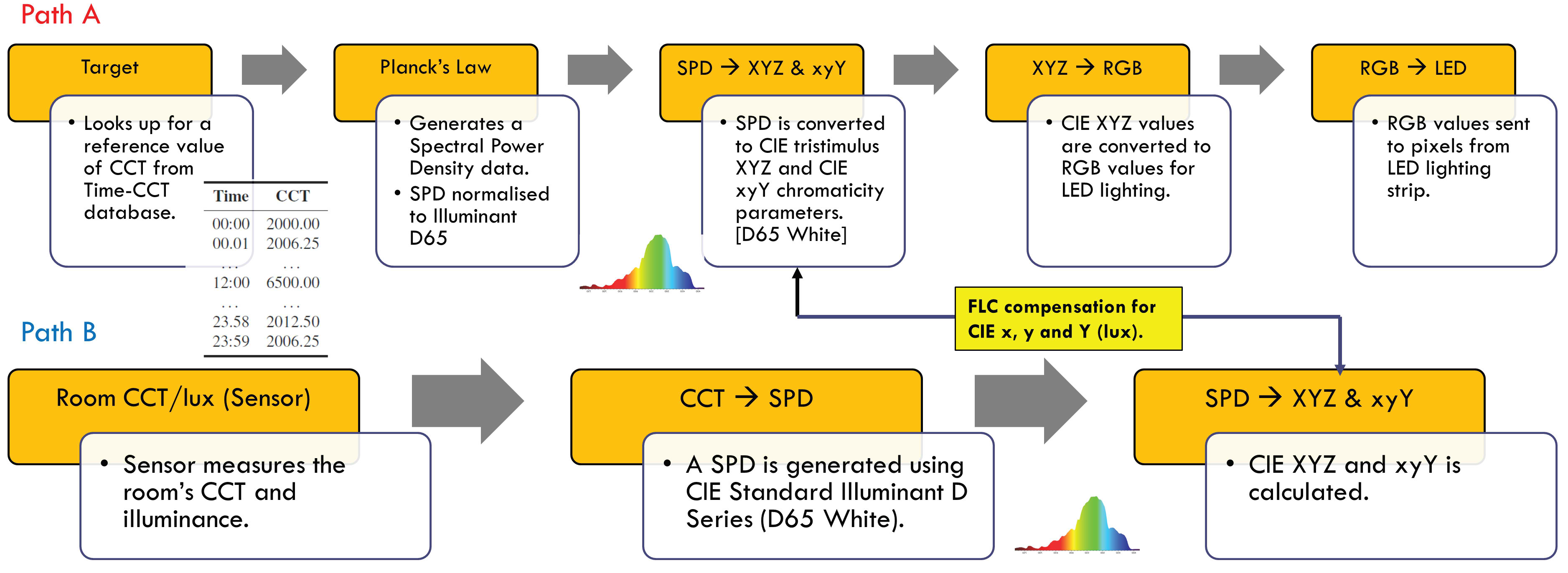Figure 5
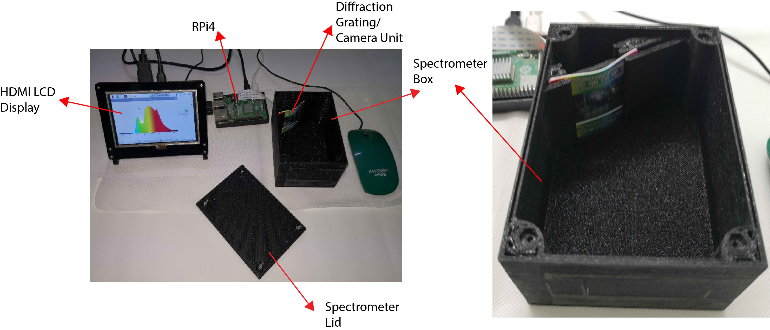Figure 6
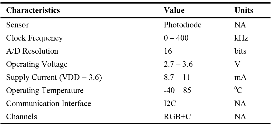Table 2
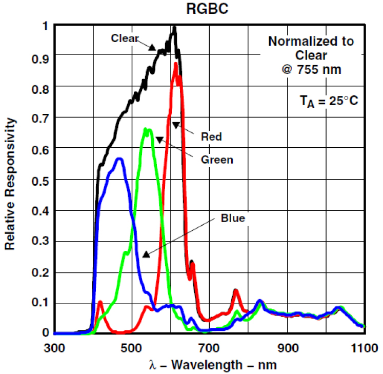Figure 7
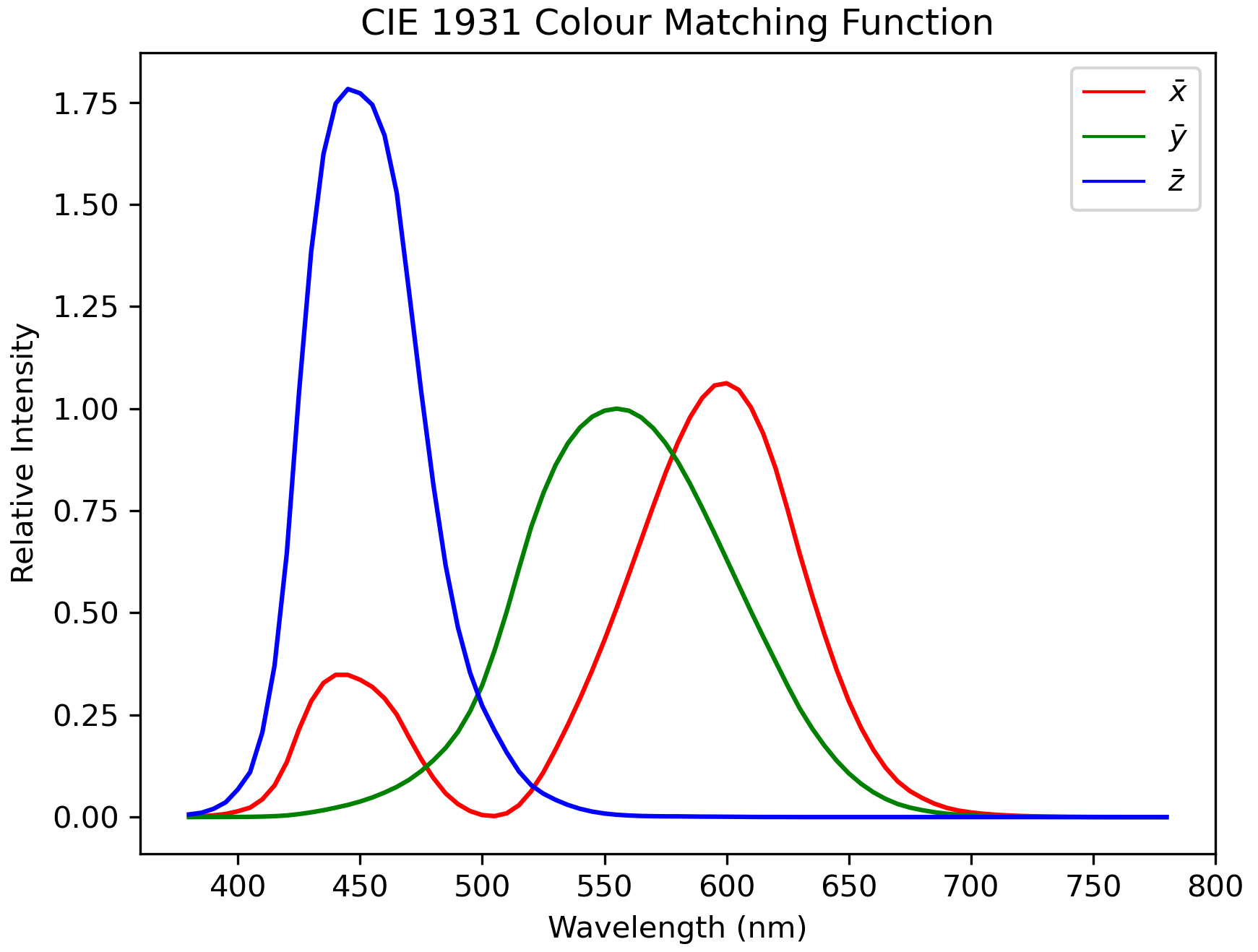Figure 8
Table 3
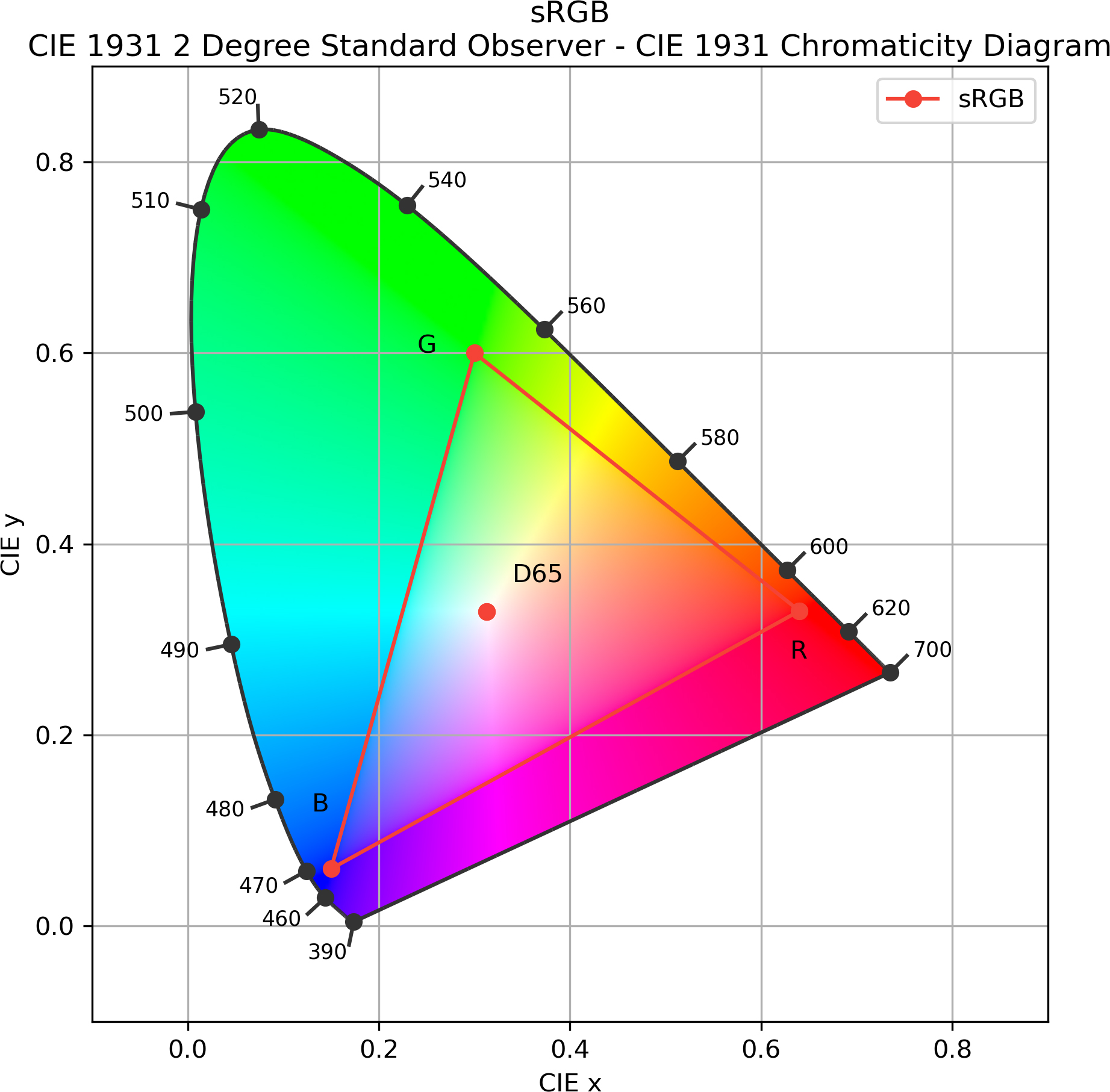Figure 9
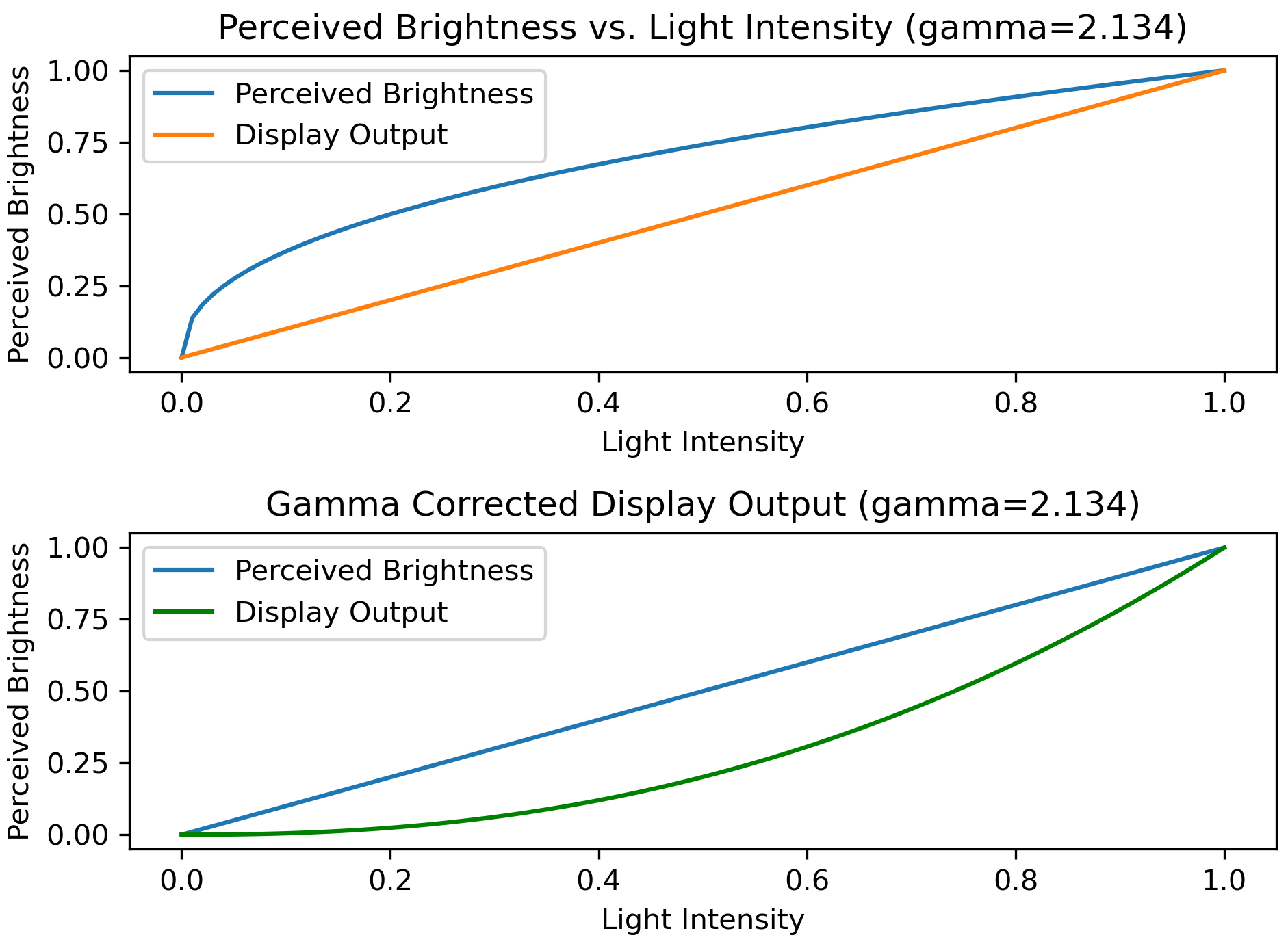Figure 10
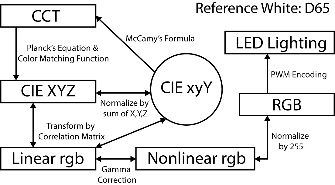Figure 11
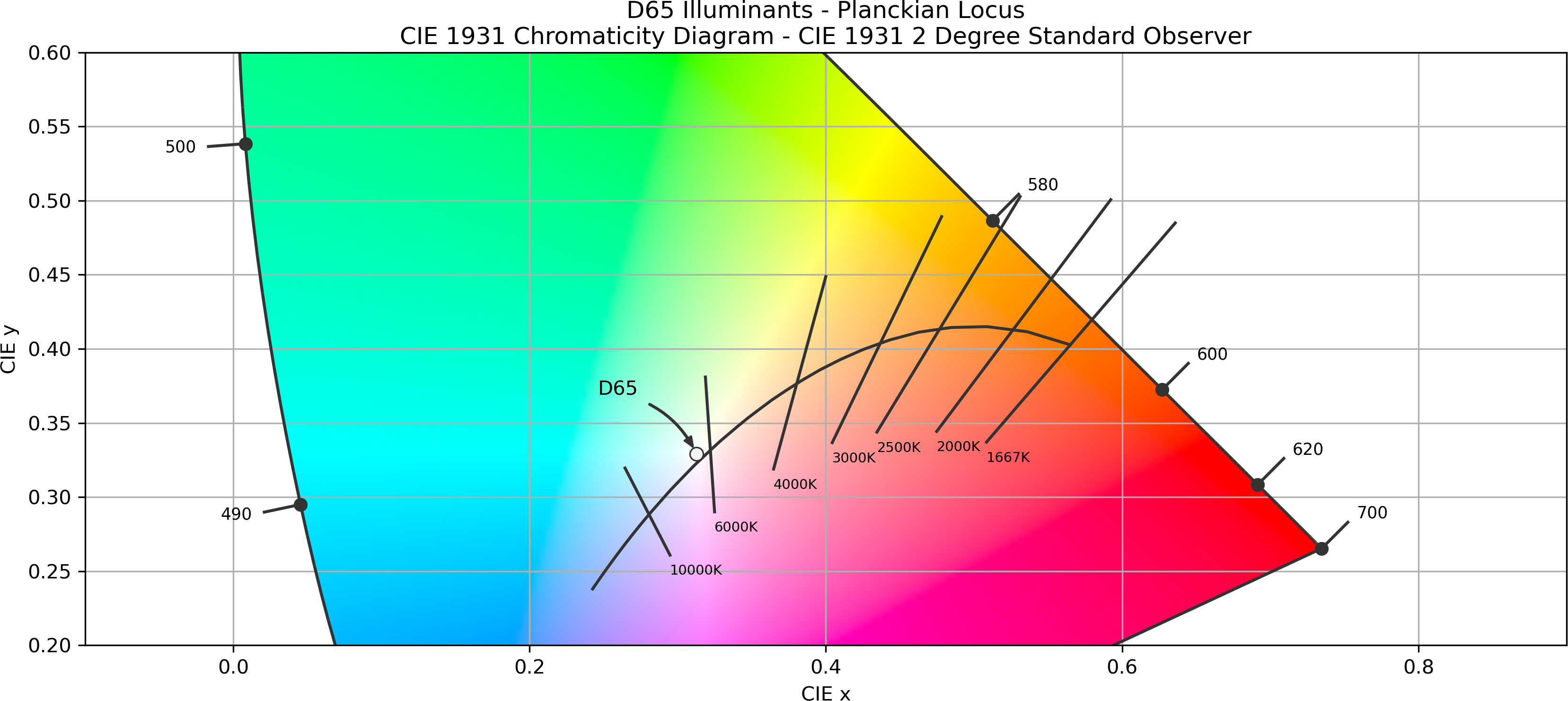Figure 12
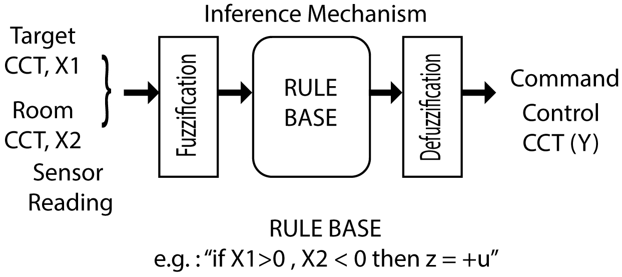Figure 13
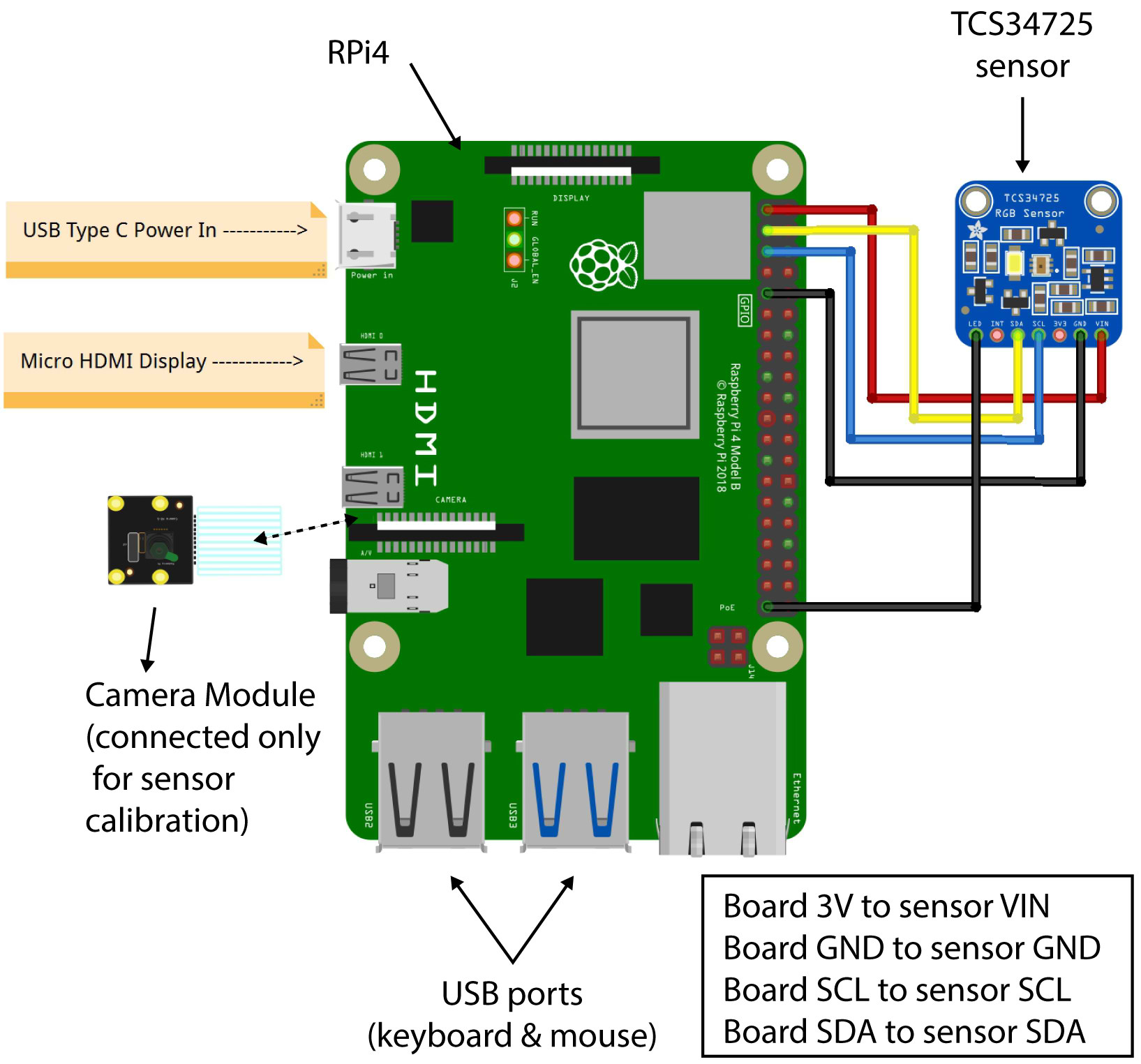Figure 14
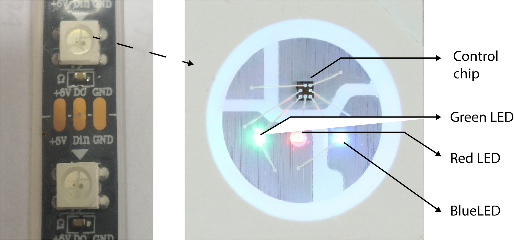Figure 15
Figure 16
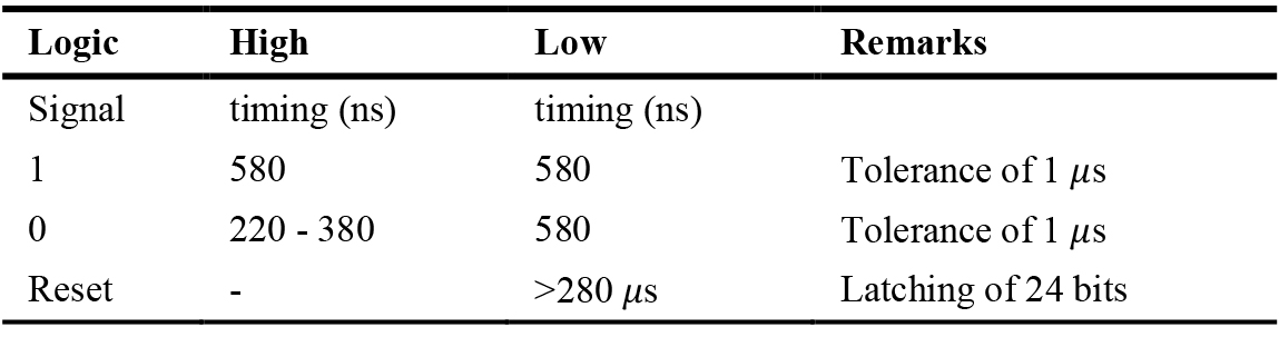Table 4
Table 5
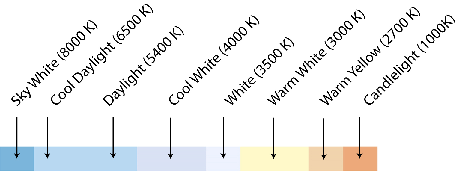Figure 17
Table 6
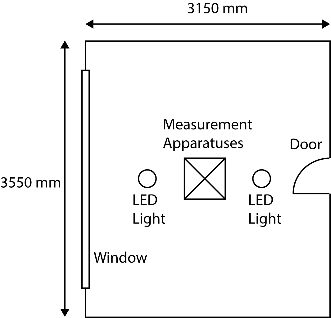Figure 18
Figure 19
Figure 20
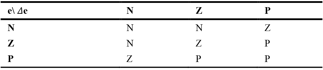Table 7
Figure 21
Figure 22
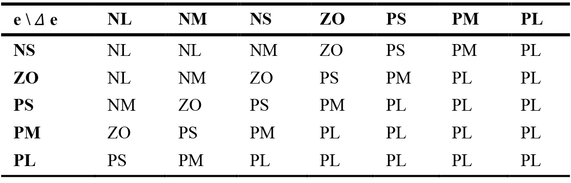Table 8
Figure 23
Figure 24
Figure 25
Figure 26
Figure 27
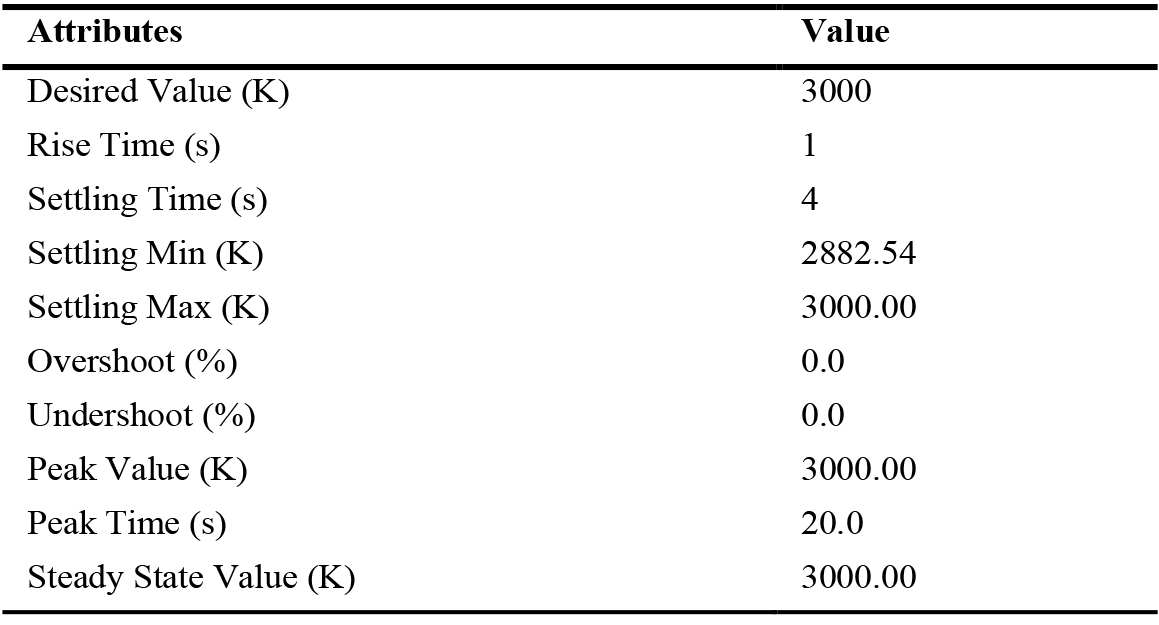Table 9
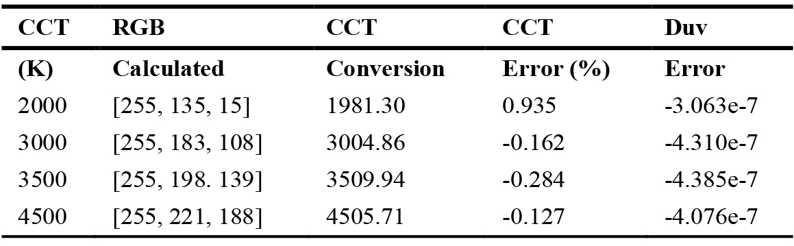Table 10
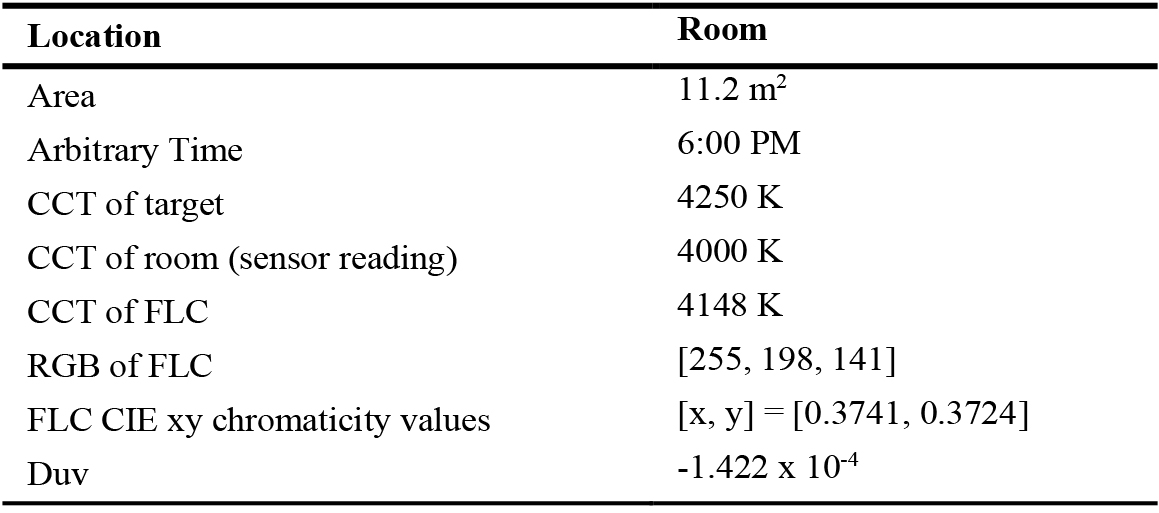Table 11
Figure 28
Figure 29
Figure 30

Abstract

This paper introduces a fuzzy logic-based circadian lighting control system using flexibility of Light-Emitting Diode (LED) lighting technology to synchronise artificial lighting with circadian (natural) lighting Correlated Colour Temperature (CCT) characteristics. Besides for vision acuity, the Non-Imaging Forming effects of lighting affect human circadian rhythms. Past works in spectrally tuning CCT or Spectral Power Distribution of lighting have used conventional Proportional-Integral-Derivative (PID) control system architecture, where the modelling process of system transfer functions was mathematically complex, especially for nonlinear systems. A methodology of regulating lighting CCT is employed in a 7×5 fuzzy logic rules matrix in a Fuzzy Logic Controller (FLC) system, to closely replicate natural lighting CCT characteristics for indoor lighting. A reference lookup table was devised to store desired CCT values arbitrarily with respect to time mark in a day, which acts as an outdoor circadian stimulus and guides the FLC. The FLC compensates for the lack of CCT in lighting space. Simulation results show acceptable CCT output values conforming to circadian lighting parameters at a time in a day compared to the lookup table targets. Deviation from blackbody curve was within ±0.003 using CCT Duv checking. The system did not produce an overshoot (0.0%) with a steady state (zero error) reached after the fourth iteration. Also, rise time was calculated to be 1 iteration. This approach could be further enhanced to cater for additional custom needs in many built environments. Future works may consider connecting more sensors to capture real-time outdoor CCT values for practical regulation.

Keywords

LED lighting, Circadian lighting, Fuzzy logic control system, Correlated colour temperature

1. Introduction

Lighting is essential at built environments. Nowadays, architects and engineers construct buildings in a closed environment with controlled and conditioned air circulated within the building. Similarly, lighting is crucial in closed settings to set the mood right for occupants in promoting well-being [1]. Designers introduce artificial lighting indoors to compensate for the lack natural light (daylight) exposure. The job and task efficiency of occupants is often affected by lighting [2]. Circadian lighting is concept of lighting which also covers daylighting introduction into building and affects the sleep-wake patterns of humans [3].

The notion of “occupant comfort” is a broad discussion area. Traditionally, building designers gave much attention to “thermal comfort.” In contrast, in today’s built-environment context, other occupant comfort parameters, such as illumination and lighting quality, indoor air quality, acoustic quality, and others, are important prerequisites in defining the well-being of occupants [4,5]. In hindsight, there is a paradigm shift where green building certifications are also taking into account circadian lighting approach while sustaining energy consumptions [6].

One of the key parameters of lighting is the Correlated Colour Temperature (CCT) of lighting that impacts occupants' well-being [7]. CCT is a single representation of lighting Spectral Power Distribution (SPD) that affects the colour (chromaticity) appearance of lighting [1,3]. The CCT varies in tandem with circadian lighting by spectrum wavelength-intensity contents. A spectrum corresponding to different CCTs has different wavelength-intensity contents. Thus, this paper aims on replicating the natural lighting’s CCT characteristics in lighting spaces through a Fuzzy Logic Controller (FLC) system via chromaticity compensation.

1.1. Circadian rhythm

Humans perceive lighting through the retina cells in the eyes, which has cone cells sensitive to wavelength peaks of red, green, and blue (RGB) colours [3]. The eye’s retina also has rod cells that guide our vision in the dark. The rod cells are sensitive to motions. Human eyes also have a fifth receptor called intrinsically photosensitive Retinal Ganglion Cells (ipRGC) [1,3,8]. These ipRGC cells are the gateway to Non-Image Forming (NIF) effects of lighting to humans and are activated by the suprachiasmatic nucleus (SCN). SCN is the trendsetter to dictate circadian rhythm in human beings and is in the brain’s hypothalamus region. NIF effects are the main catalyst that influences melatonin and cortisol hormone production in human bodies [3,8,9]. In daytime, our body requires the cortisol hormone to be active or alert. In contrast, melatonin is a hormone that triggers sleep (rest) at night. Figure 1 depicts the relative hormonal markers in the human body for 24 hours cycle.

Figure 1

Fig. 1. Relative markers of the human circadian rhythm [3].

1.2. Fuzzy logic control system

Fuzzy logic is an intelligent decision-making approach used in different fields such as engineering, share markets, and others areas [10]. This logic-based strategy has its advantage when scarcity (fuzziness) is concerned. Fuzzy Logic Controllers (FLC) are similar to conventional control system, but it applies fuzzy logic theories. Engineers can design an FLC to interpret the proportions and quantities of human linguistic references. For example, a fixture’s lighting brightness (luminance) output can be configured to be pre-set at settings “low,” “medium,” and “high.” Many human expectations and references that are associated with electrical parameters can be optimised in aggregated-like calculations for decision making through Fuzzy Logic methodology [11]. In Fuzzy Logic applications, the linguistic references can be quantified between 0 and 1 for electronic controllers to interpret [12]. The quantification’s dimensions are also referred to as membership functions. After its concept introduction during the 1960s, engineers preferred to use fuzzy logic in control systems when complexity (non-linearity) in system modelling were involved [13,14]. FLCs are cheaper and easier to implement compared to conventional Proportional-Integral-Derivative (PID) control systems [13]. Meaning, if the relationship between input and output is nonlinear, extensive mathematical computations are needed to yield an output. That is, higher degree relationship functions become more extensive for computers to process, which leads to more power consumptions.

Any control system may be in the form of either open-loop or closed-loop [15]. The key benefit of using a closed-loop feedback system is that it minimises external disturbances introduced into system plants (process) to achieve greater precision at control output [16,17]. Unregulated light sources and the controller’s (or plant) inherent nonlinearity (noise) can cause disturbances to a control system.

From Fig. 2, the choice of a controller block may be either a classical proportional–integral–derivative (PID) controller, FLC or a hybrid PID-FLC controller. In comparison, when programmed to other nonlinear systems, the FLC module may not require extensive re-tuning to achieve desired results based on the platform [10,13]. Most FLC does not require re-tuning since an FLC control system does not need to know the transfer function of its plant during the designing phase. Transfer function modelling process is the input-output mapping of a control system. If the controller block in Fig. 2 is substituted with an FLC block, it becomes a closed-loop FLC control system. However, an FLC system needs expert guidance or experience to tune the system by choosing a suitable fuzzy rule matrix. Therefore, if the designer understands the expected behaviour of the system well, the weightage of integrating fuzzy logic concept in the control system will be minimal [11,18,19].

Figure 2

Fig. 2. Generic closed-loop control system block diagram.

King et al. [13] used a fuzzy logic algorithm in controlling a boiler and a steam engine. The heat input to the boiler was used to control the boiler pressure, and the steam engine speed was controlled by adjusting the throttle opening at the input of an engine cylinder. The results obtained show that complex process can be effectively controlled using trial-and-error rules based on fuzzy statements. The system’s response was better than conventional PID controllers, which had a rippling response before reaching a steady state.

Singhala et. al [14] used FLC to create a temperature control system that heated an electric heater in proportions to the temperature reduction in a test room. Excessive heat in the room was compensated by a fan attached to the system. Like the design in this paper, Pulse Width Modulation (PWM) output is generated to control the power generated to the heater and fan. Their concluding note stated a successful application of FLC to control the room temperature to its desired value without modelling the system’s transfer function.

Almatheel and Abdelrahman [20] managed to regulate the speed of a DC motor with an FLC and compared its results to the conventional PID controller. However, they conjured an intensive forty plus fuzzy set of rules matrix (7×7 fuzzy inputs and 7 fuzzy outputs) to define the system’s behaviour. The speed of the DC motor output has a nonlinear relationship to its input current. Extensive mathematical modelling is required to generate the transfer function representing process dynamics for a PID controller compared to an FLC where experience is needed to guide the output. The results show that the FLC response has minimum transient and steady-state parameters, which shows that the FLC is more efficient and effective than a PID controller.

Liu et al. [21] applied the concept of fuzzy logic in their illuminance control system. A balanced illuminance output was generated in their application between outdoor and indoor lighting to conserve energy utilisation. Specifically, indoor illuminance level was measured on work tabletops. An FLC was designed in which the daylight contribution and user lighting comfort factors were considered and optimised. User required minimum illuminance level was set as a threshold that the FLC must produce near worktables, whereas other circulation areas in the room did not matter. Their experimental data showed that lighting levels on worktables remained optimal above the threshold level, despite changes in outdoor daylight patterns. Through their method, energy consumption was reduced when illumination was decreased at non-essential areas.

1.3. Gaps and opportunities from past works

In the scope of lighting, beyond the control of illuminance, where most standards and regulations focus on, several works have been done to spectrally tune lighting through SPD replication which results in CCT variance. Multiple approach of mixing CCTs from known CCT light sources through lighting control systems was also utilised. The SPD replication method is more accurate to represent circadian lighting as it affects the NIF effects through the various wavelength contents in the lighting source [3]. The CCT mixing methodology, may not represent faithfully the desired lighting in terms of wavelength-intensity content, as various combinations of colours can produce the same CCT. However, studies basing on SPD generation requires spectrometers as sensors.

Chen et al. [22] varied CCT through a combination of two light sources of known CCT 2700 K and 5000 K. Through PWM control, the final lighting, average CCT, was tuned by mixing the intensities of both sources. However, the system was designed in an open-loop PID architecture, where the final CCT output may have noises or errors embedded. Similarly, Lee et al. [23] also managed to control CCT through a nonlinear empirical PID open-loop model that uses bicolour white Light-Emitting-Diode (LED) system. Buso et al. [24] used three LED lighting arrays to manage CCTs by individually controlling LED arrays of colour red, green and blue. Kim et al [25], meanwhile, simplified the CCT determination through RGB weighted average computation. In contrast, the control mechanism dealt with CCT like Chen et al., Lee et al and Kim et al. works but does not accurately replicate SPD. Gao et al. [26] focused his work on minimising the blue wavelength contents from lightings that has health concerns by optimising the CCT through chromaticity coordinate balancing. Meaning, choosing combinations of other colours without the blue contents to reach to the same desired CCT. Muthu et al. [27], in his work, described the issues escalating when using LED lighting to produce white light by solving them in a closed-loop system that balances the output lighting to be near the white light region (near the blackbody curve). Recently, Chew et al. [17] designed a closed-loop control system that regulates the CCT through SPD compensation. Table 1 summarises the application of control system in lighting CCT management.

Table 1

Table 1. Comparison of lighting CCT management control system.

From Table 1, most of the past works have used open loop control scheme. Only a few relating studies that regulated CCT or SPD that utilised closed loop architecture. Both closed loop in the latter works were using classical PID architecture. Since, FLC system have some advantages over PID system such as application ease and cost, this paper aims to present a design of a control system utilising Fuzzy Logic Controller to vary and regulate CCT given the importance of circadian lighting introduction into lighting spaces.

2. Methodology

The LED lighting control system consists of three modular blocks, as illustrated in Fig. 3. The first module, the Sensor Module, comprise of a TCS34725 RGB (Red, Green, Blue) colour sensor unit. The second module houses a minicomputer for data processing, and the third module is the LED lighting device for lighting output. This research will construct a prototype by connecting the three modules for testing and simulation later.

Figure 3

Fig. 3. Block diagram of modules for the lighting control system.

In the control system architecture illustrated in shown in Fig. 4, there are two main pathways of colourimetry processing. In the first pathway, a CIE Standard Illuminant D SPD will be generated referring to the desired (target) CCT using the Commission Internationale de l’Eclairage (CIE) colour space colourimetrics [17,28,29]. Here, desired CCT values refers to an arbitrary value arranged and coordinated with natural lighting CCT and time of the day. Through the second pathway, colourimetry parameters are calculated using the measured raw data from the RGB colour sensor. The RGB sensor data are sent to the data processing module. In the data processing module, the corresponding CIE xyY chromaticity and XYZ tristimulus values will be determined for compensation process from both pathways. Finally, the compensate RGB output is determined from the CIE tristimulus XYZ values of the compensate CCT before sending it to the LED lighting luminaires. The RGB values are equivalent to [0-255] pixel bit values normalised between 0 and 1. Figure 5 shows the process flow of the control system on a block diagram. Conversions between CCT, CIE XYZ and RGB values are part of colourimetry topic which will described in section 2.2.

Figure 4

Fig. 4. Block diagram of closed loop with FLC system.

Figure 5

Fig. 5. Process flow of lighting control steps.

Note: In Fig 4, CCT is Correlated Colour Temperature, SPD is Spectral Power Distribution, XYZ are the CIE tristimulus values, xyY is the CIE chromaticity coordinates coupled with Y Luminance, RGB represents Red, Green, Blue and LED is Light Emitting Diode.

An FLC control system was chosen due to its reproducibility when ported to other systems. Besides, it does not require the system process transfer function derivation [10,13,14]. Meaning, when programmed to other nonlinear plants and controllers (microprocessors or microcontrollers), the FLC module may not require extensive re-tuning to achieve desired results based on the platform. Tuning means guiding the FLC through a set of fuzzy rules matrix like PID system tuning.

The FLC takes two inputs in error and change in error (delta error). The error function, , is the algebraic subtraction of reference, function, and the output, . The function, , signifies the amount of correction (compensation) that needs to be adjusted for the output, function to match the input reference, . The change in error, signifies the direction the error control action should undertake by either increasing or decreasing the correction action proportionally. The amount of correction and direction follows the rules that is set by the designer.

Additionally, the sensor requires calibration before being utilised to output accurate measured CCT values. The sensor calibration step involves comparing the CCT value measured from the sensor and a spectral irradiance produced by a spectrometer. The spectrometer was also self-developed using 3D printing technology as shown in Fig. 6.

Figure 6

Fig. 6. 3D printed spectrometer for calibration.

In this paper, the calibration step is not focused as its detailed description is another topic altogether. However, to explain briefly, the CCT of a light source from the spectrometer is determined by generating the light source’s spectral power distribution (SPD) in a field of view (FOV) of the RGB sensor. It is then compared to the CCT readings of the RGB sensor module and hence calibrated using a statistical regression tool to produce a sensor characteristic mapping function.

2.1. Materials for Prototype

In Fig. 3, the Data IO Processing module is a minicomputer. The design presented in this article utilises the Raspberry Pi 4 (RPi4) minicomputer with Linux Debian based Operating System, Raspbian [30]. Python scripting language is used for all mathematical calculations, coding, and simulation. The super small size characteristic of the RPi4 allows all the codes to be packed into a single credit card-sized board. Thus, lighting monitoring, control, and regulation could be compactly executed at a corner of an indoor space. Note that the minicomputer RPi4 and the sensor TCS34725 are chosen in this design based on availability, cost, and online support community. Any other similar devices may be used. Table 2 shows the characteristics of the TCS34725 colour sensor whereas Fig. 7 presents the spectral response [31].

Table 2

Table 2. TCS34725 RGB colour sensor characteristics.

Figure 7

Fig. 7. Spectral response of TCS34725 RGB colour sensor [31].

2.2. Colourimetry: SPD to XYZ, CCT, RGB Calculations and Conversions

The CIE colourimetry space is used for the conversion from one dimension to another. There are few variations of CIE colour space. In this design, the “CIE 1931 2 Standard observer” colour space is used as a platform for conversions due to widely available supporting literature [17,28,33]. After measuring the CCT of an indoor space using the sensor, an SPD is generated using the CCT value using the Planckian function. However, a simpler equation exists to model natural daylighting as opposed to using Planckian equation. The former method was chosen as in future, the sensor can be upgraded to spectrometric sensor which could measure the spectral irradiance accurately as compared to TCS34725 sensor which only converts the RGB response to CCT. Planckian equation to generate SPD is done by using Eq. 1.

\[ B\left(\lambda;T\right)=\frac{\frac{2hc^2}{\lambda^5}}{e^\frac{hc}{\lambda k_BT}-1} \]

where:
B(λ;T) – spectral energy emitted per unit of time, area, and solid angle (W m^-3 sr^-1)
h – Planck constant (6.63 x 10^(-34) Js)
T – colour temperature of the body
λ – corresponding wavelength
c – speed of light (3.00 x 10⁸ m/s)
k_B – Boltzmann’s constant (1.38 x 10^(-23) J/K)

Colour matching in the RGB space uses the CIE standard illuminant D65 as the reference white. When SPD data for a light source is available, the first step is to convert them to CIE tristimulus XYZ values. The step is performed by integrating the product of a light source’s SPD data and the CIE colour matching function components. The CIE colour matching function is a set of red, green, and blue intensity values mapped to its wavelengths, as shown in Fig. 8. Fundamentally, the mapping function is a generic colour sensitivity perception of human eyes [34].

Figure 8

Fig. 8. CIE 1931 2° colour matching function.

When we have arbitrary SPD (spectrum) data, it can be converted to be represented in CIE XYZ tristimulus values as in Eq. 2, 3 and 4. The XYZ values are essential, as it describes the ratio of colour mixing of primary red, green, and blue colours to render a specific output colour.

\[ X=\int P\left(\lambda\right)\ x\left(\lambda\right)d\lambda \]

\[ Y=\int P\left(\lambda\right)\ y\left(\lambda\right)d\lambda \]

\[ Z=\int P\left(\lambda\right)\ z\left(\lambda\right)d\lambda \]

The X, Y, Z parameters can be normalised to be represented in cartesian coordinates, called CIE chromaticity coordinates, as in Fig. 9. However, by doing so, the relative brightness (luminance) information from the SPD is lost. The chromaticity coordinates (x, y) represent colour in 2D space and are calculated through Eq. 5, 6 and 7.

\[ x=\frac{X}{X+Y+Z} \]

\[ y=\frac{Y}{X+Y+Z} \]

\[ z=\frac{Z}{X+Y+Z}=1-x-y \]

Figure 9

Fig. 9. CIE 1931 2° chromaticity (x,y) diagram.

The RGB value corresponding to an SPD is determined through further conversion from the CIE tristimulus XYZ or xyY coordinates data as Eq. 8. The RGB values are within the 0-1 range. Another distinction must be made to update the uniform RGB values (0 to 1.0) to the digitised RGB values (0-255) when transmitting to digital systems such as LED lighting systems. Geometrically, Eq. 8 maps any arbitral SPD (or CCT) into an RGB gamut. Gamut refers to a space of achievable colours in a modern display colour system by mixing red, green, and blue in the CIE chromaticity diagram. The standard RGB (sRGB, ITU-R BT.709) gamut is used in this design as it closely resembles the LED luminaires property of storing 8-bit integers per colour channel [35]. Table 3 shows the RGB primary data for the sRGB colour system. The sRGB gamut is represented by the RGB triangle depicted in Fig. 9. The standard illuminant white D65 is marked in the middle of the triangle at x = 0.3127 and y = 0.3290.

\[ \left[\begin{matrix}x_r&x_g&x_b\\y_r&y_g&y_b\\z_r&z_g&z_b\\\end{matrix}\right]\left[\begin{matrix}r\\g\\b\\\end{matrix}\right]=\left[\begin{matrix}x\\y\\z\\\end{matrix}\right] \]

The x_(r/g/b), y_(r/g/b) and z_(r/g/b) from Eq. 8 represents the transformation matrix values referring to D65 standard white’s chromaticity coordinates as in Table 3.

Table 3

Table 3. Chromaticity coordinates of primary colours for the sRGB colour system.

The human visual perception of brightness is nonlinear [36]. If B is the light intensity produced by a luminaire and L is the perceived brightness, the amount of light entering our eyes is given by an inverse exponential function as in Eq. 9 where γ is a numerical skew factor. At high luminance (brightness) value, human eyes do not detect the minor variations as depicted in Fig. 10 (top-plot) due to the nonlinearity [37].

\[ B=L^\frac{1}{\gamma} \]

Figure 10

Fig. 10. Lighting brightness perception of human eyes.

Eq. 10 shows the derivation of perceived brightness for a three-colour system of RGB luminaire. The transformation in Eq. 10 is called gamma correction. Gamma correction is done to lighting RGB values to match it to the characteristics of human eyes, Fig. 10 (bottom plot) [37].

\[ B=\left(R^\gamma+G^\gamma+B^\gamma\right)^\frac{1}{\gamma} \]

To transform the rgb values from Eq. 8 into human-perceivable brightness fluctuations for any RGB colours, Eq. 11 is applied to the rgb values [28].

\[ \atop V= \cases{ 12.92, if\ v≤0.0031308 \cr 1.055v^{\frac{1}{2.4}}-0.055, if otherwise } \]

Alternatively, the inverse of gamma-correction is:

\[ \atop V= \cases{ \frac{V}{12.92,} if v≤0.04045 \cr ({\frac{V+0.055}{1.055}})^{2.4}, if otherwise } \]

V is the gamma-corrected r, g, b values into RGB, whereby rgb are linear values and RGB are nonlinear values referring to Fig. 10 (bottom-plot) as in Eq. 13 and 14.

\[ v\in{r,g,b}, linear \]

\[ V\in{R,G,B}, non-linear \]

Once gamma correction is done, the RGB could be correlated to 0-255 values. To convert RGB values back into CIE tristimulus XYZ values, the inverse gamma correction is applied first.

When an SPD is converted to CIE XYZ tristimulus values, the intensity-wavelength data and its relative luminance value are lost, making it mathematically extensive to inverse the operation. However, the CCT of the SPD can be recalculated using McCamy’s formula. Since the range of the CCT is small (2000 K to 6500 K) in this design, then McCamy’s third-order polynomial function, as in Eq. 15, is applied by utilising the CIE xy chromaticity coordinates [38].

\[ CCT=449.0n^3+3525.0n^2+6823.3n+5520.33 \]

where,

\[ n=\frac{\left(x-0.3320\right)}{\left(0.1858-y\right)} \]

The CCT is not linearly related to CIE XYZ tristimulus values or the CIE xy chromaticity coordinates, as Eq. 11, Eq. 15 and Eq. 17 shows. Thus, at any measurement instance, the CCT of the lighting space must be compensated to the desired CCT by the CIE xy chromaticity coordinates first and hence converted R, G, B component values after. Therefore, the working domain for compensation is in the CIE xy chromaticity coordinates domain (or CIE xyY, to retain luminance information). The compensation techniques are the basis for regulated lighting, as depicted earlier in Fig. 5. The compensations are done in the workspace of the CIE xyY chromaticity environment, as illustrated in Fig. 11.

\[ CCT_{desired}\neq CCT_{room}+CCT_{compensation} \]

Figure 11

Fig. 11. Workspace environment for colourimetry.

Also, Fig. 11 further highlights the conversion process of colourimetry parameters. Each conversion process is stated beside the relationship arrows in the figure. CCT values measured from the sensor or read from Ssection 2.5 are reduced to CIE xyY parameters to be processed by the control system. Based on the CIE xy parameters, compensation values for lighting CCT regulation will be determined from the FLC operations. The resulting compensated CIE xy will be used to reconstruct compensation SPD to be output by the lighting device. The process will be repeated until steady state is achieved.

The CCT value sets are represented by the iso-thermal lines in the CIE 1391 chromaticity chart as in Fig. 12.

Figure 12

Fig. 12. Planckian locus on the CIE 1931 chromaticity diagram with Standard Illuminant D65.

From Fig. 12, note that there are multiple RGB combinations to produce a CCT. Therefore, after determining the CCT value, a check on the deviation of the CCT value from the blackbody curve is done using the Duv calculation [39,40]. This check is to ensure that the CCT calculated is in the white colour zone of Fig. 9 as marked D65. A Duv range between -0.003 and +0.003 is the minimum requirement to pass the check. In other words, a Duv check determines how far the calculated CCT is from the blackbody curve. Eq. 18 to Eq. 23 shows the steps and derivation to arrive at a Duv value starting from the CIE xy coordinates.

\[ u=\frac{4x}{-2x+12y+3} \]

\[ v=\frac{6y}{-2x+12y+3} \]

With constants, k₀=-0.471106, k_1=1.925865, k₂=-2.4243787, k_3=1.5317403, k_4=-0.5179722, k_5=0.0893944, k_6=-0.00616793, then:

\[ L_{FP}=\sqrt{\left(u-0.292\right)^2}+\left(v-0.24\right)^2 \]

\[ a={\mathrm{cos}}^{-1}\left(\frac{u-0.292}{L_{FP}}\right) \]

\[ L_{BB}=k_6a^6+k_5a^5+k_4a^4+k_3a^3+k_2a^2+k_1a^1+k_0a^0 \]

therefore,

\[ Duv=L_{BB}-L_{FP} \]

The above formulae are the foundations of colourimetry. They are widely available in various programming languages as a third-party library. This design will use the Colour Science library for Python, which already has pre-programmed the formulas for external use [41].

2.3. Fuzzy logic control mechanism and compensation

Further dissection of the Fuzzy Logic Controller block in Fig. 4 demonstrates the inferencing process occurring within it, as shown in Fig. 13. If the expert intuition is not incorporated into the system, a continuously running control regulator system is not intelligent. The Fuzzy Logic tool’s inference mechanism is a method that aggregates the inputs to predict a user-guided output based on his experiences. User-guided means a designer can alter the speed and direction of output change, having known the expected response. In this design, the open-loop response was used to guide the closed-loop output.

Figure 13

Fig. 13. Fuzzy Logic inference mechanism.

The inputs to the FLC are error (e) and change of error (Δe). Both variables are distributed with corresponding labels into various fuzzy sets. The fuzzy variables are defined based on the required values in the discourse universes. These steps are also performed for the control action operation, labelled as Δu in Fig. 4.

Once the input and output have been fuzzified, fuzzy rules are developed based on the user’s intuitive knowledge and experience (also trial and error). The system is then simulated to store the rule database in the controller’s memory. After assessing all the input and output choices in the discourse universe, the FLC builds a lookup table (LUT) for future uses, rather than recalculating them in each regulating loop. Subsequent FLC processes are executed within milliseconds [19].

When the defuzzied output Δu or z* is available, the FLC control system sends the signal to the plant (LED lighting strip), as in Fig. 4. The LED lighting luminaire contains the actuator (LED driver) and the LEDs. Intrinsic noises and external lighting introduced as disturbances by the LED driver module are taken care of by the FLC through error correction. The control algorithm is implemented in practical applications in a continuous loop to regulate the lighting output.

In this design case, the inputs to the FLC are the room’s light and the target’s light spectrum. FLC distributes these variables into corresponding values on various fuzzy sets. Then the fuzzy variables are defined based on the required values in the discourse universes. These steps are also performed for the output. Eq. 24 mathematically represents an input/output variable in fuzzy membership functions.

The FLC can predict output based on the rules defined by users. This design utilises the Mamdani Max-Min Inferencing method to generate an output membership activity. They are known as Mamdani’s max-min compositional operator [13]. RPi4 merges the activated fuzzy variables using a maximum operator to accomplish this in the control system with the max-min compositional operator results. Aggregation is another name for this step.

\[ F=\sum_U μFX/X \]

RPi4 sets the input values (universe of discourse) for circadian lighting control between a normalised value of 0 and 1. Hence, CCT can be normalised to between 0 and 1 when inferencing executes within the FLC block.

Once the merged membership functions for output is determined, the defuzzification technique is applied to get a crisp (actual) output. This design will use the centroid defuzzification method as it is the most popular and physically appealing technique. Eq. 25 shows the formula for the centroid defuzzification technique.

\[ z^\ast=\frac{\sum\mu_z\left(z\right)\cdot z}{\sum\mu_z\left(z\right)} \]

Note: In Eq. 25, z* is the crisp output value. μ_z are the output membership values, and z is the crisp value corresponding to the membership value.

The methods described for FLC are utilised using Python open-source library scikit-fuzzy [19,42]. Figure 14 shows the schematic connections for the control system drawn using Fritzing CAD software.

Figure 14

Fig. 14. Lighting control system schematic diagram.

2.4. LED lighting luminaires

RGB tuneable LED strips are used for their versatility in operation and design. LED strips are chosen where a wide variety of colours could be rendered within the CCT range. Each strip consists of WS2812B surface mounted technology (SMT) LED chips. The WS2812B LED strip is a voltage-controlled constant-current driver type [43].

Colour variation is controlled by driving the high-frequency PWM signal through the control pin. The control PWM signal is manipulated by adhering to the procedures defined in the device’s datasheet to generate the desired output.

LED lighting strips with a built-in driver such as WS2812B are addressable. LEDs can be managed individually for colour and brightness levels using this addressable property. For example, sixty distinct colours can be made with 60 LED chips on a one-metre-long strip.

Each LED chip on a strip, denoted as a pixel, contains three sub-LEDs of red, green, and blue fabricated together, as shown in Fig. 15. Each pixel is 5 mm x 5 mm in size and powered by a 5 V DC power supply. It also includes a built-in mini-circuit control driver. Each LED’s colour and brightness are controlled via serial communication protocol, where a 24-bit frame data packet is sent in PWM format. The 24-bit frame has three channels of one byte per channel for colour control (R, G, B). The data frame is encoded by the GRB sequence, as shown in Fig. 16 [43].

Figure 15

Fig. 15. WS2812B closeup view.

Figure 16

Fig. 16. GRB data frame per pixel (24 bits).

For each byte (8 bits) of data, for example, green channel, G7 is the most significant bit compared to G0, which is the least significant bit for brightness value. A Non-Return Zero (NRZ) encoding scheme is used in the serial interface, where both the 0 and 1 signal is characterised in a fixed frequency square wave by varying the duty cycle. The difference between 0 and 1 is the time duration for the PWM signal high and low state. For a duty cycle of 1.25 μs long (800 kHz), the required holding time to form a “low-0” signal and a “high-1” signal is tabled in Table 4. The 24-bit frame can only control a single pixel. If there are 12 pixels along a strip, then 12 x 24 bits = 288 bits are sent in a packet. Each 24 bit is separated by a latching timer where the data line holds a low signal for 280 μs, indicating a complete pixel per strip. The low signal of 280 μs is critical for latching purpose before receiving the next data frame.

Table 4

Table 4. PWM control timing requirements for WS2812B LED strip.

By combining the data frames, the LED pixels can display 256 x 256 x 256 = 16, 777, 216 colours. Depending on user demand, the maximum value of 256 [0-255] bits is trimmed to add brightness control for each pixel. The pixels would have a lesser colour choice in doing so. For example, if max brightness is 100% (255), setting a 50% brightness value will cap the maximum bits per sub-pixel to 127 bits, resulting in 127 x 127 x 127 = 2,048,383 colours. However, the source’s colour property (chromaticity) is still preserved due to the RGB mixing ratio, and only causing the brighter variants of the colour lost. As there are only 5000 distinct colour variations in the range of 2000 K to 7000 K CCT, this restriction does not concern the circadian lighting through CCT regulation. Energy saving is also observed because the trimmed PWM duty cycle has fewer high bits, resulting in lower power consumption.

2.5. Circadian lighting stimulus for desired (target) CCT

An ideal lighting CCT control system shall have at minimum two sensors acting as reference (desired or target) and output measure feedback. They shall be placed, one externally (outdoor) to capture actual outdoor lighting spectrum and another installed indoors for lighting space measurements. However, due to the hardware limitation of the RPi4 minicomputer , which only allows for connecting single sensor for the serial interface, an arbitrary reference lookup table in the form of database was constructed as Table 5. The limitations are further discussed in section 4.0.

Table 5

Table 5. Database extract of arbitrary time-CCT mapping.

A database mapping timeframe to CCT is initially generated and stored in the computer’s memory. The variance of CCT from 00:00 hours to 23:59 hours is extrapolated in increasing and decreasing fashion between 2000 K to 6500 K, and back to 2000 K. An extract of the database shape is tabulated in Table 5. The range of 2000 K to 6500 K is chosen to conform to McCamy’s formula’s accuracy (2856 K to 6500 K) and practical reasons [38,44].

The above database signifies an assumption and evenly arranged CCT’s circadian sync to a time-mark in one day. Although, the values in Table 5 does not represent any real-life occurrence, they are deemed to be sufficient for simulation purpose based on the assumption that evenly spread CCT and time domain covers all extremes. However, the mapping of time-CCT in the Table 5 may be altered and changed based on geographical and seasonal variations or substituted with another sensor. In addition, the assumption does not affect the functionality of the proposed lighting control system. The ability to produce lighting and illuminate an indoor space with the circadian-synced CCT emphasises occupant comfort.

Figure 17 depicts an example of a typical CCT range offered by a lighting manufacturer which are available in the market today [45]. However, according to EN12464-1 standard, a more accurate labelling of CCT and their labelling are defined as summarised in Table 6 [46]. Although the inability of our vision to be sensitive to diverse colours in that range (Fig. 17), the critical factor is the wavelength content of the light spectrum, which affects the mood, comfort, and well-being of the user - the NIF effects of lighting.

Figure 17

Fig. 17. CCT and their conventional labelling by OSRAM SYLVANIA.

Table 6

Table 6. EN12464-1 Correlated Colour Referencing.

2.6. Simulation procedure

Simulation is done by evaluating the performance of the designed control system using Python scripting software. The dynamics of the FLC system is programmed into the RPi4 and data stored in its memory is used for external analysis [19]. The test apparatuses are placed in the middle of a test room as shown in Fig. 18 [32]. The sensor would measure the ambient lighting in the room regardless of time and architectural properties. When the system has completed several runs of compensation, the data, such as SPD and CCT is extracted from the RPi4 and analysed on a separate computer.

Figure 18

Fig. 18. Test apparatus in the test room.

The stored data are the sensor measurements, time-CCT database, FLC compensated CCT and chromaticity coordinates. These values are then plotted on charts to assess the control system performance.

3. Results and analysis

3.1. Hardware

For the purpose of evaluating the design concept, hardware was constructed. Figure 19 shows the complete apparatus set up for testing. They are components from the Fig. 3 spanning three modules, namely sensor module, data processing IO module and LED lighting output module.

Figure 19

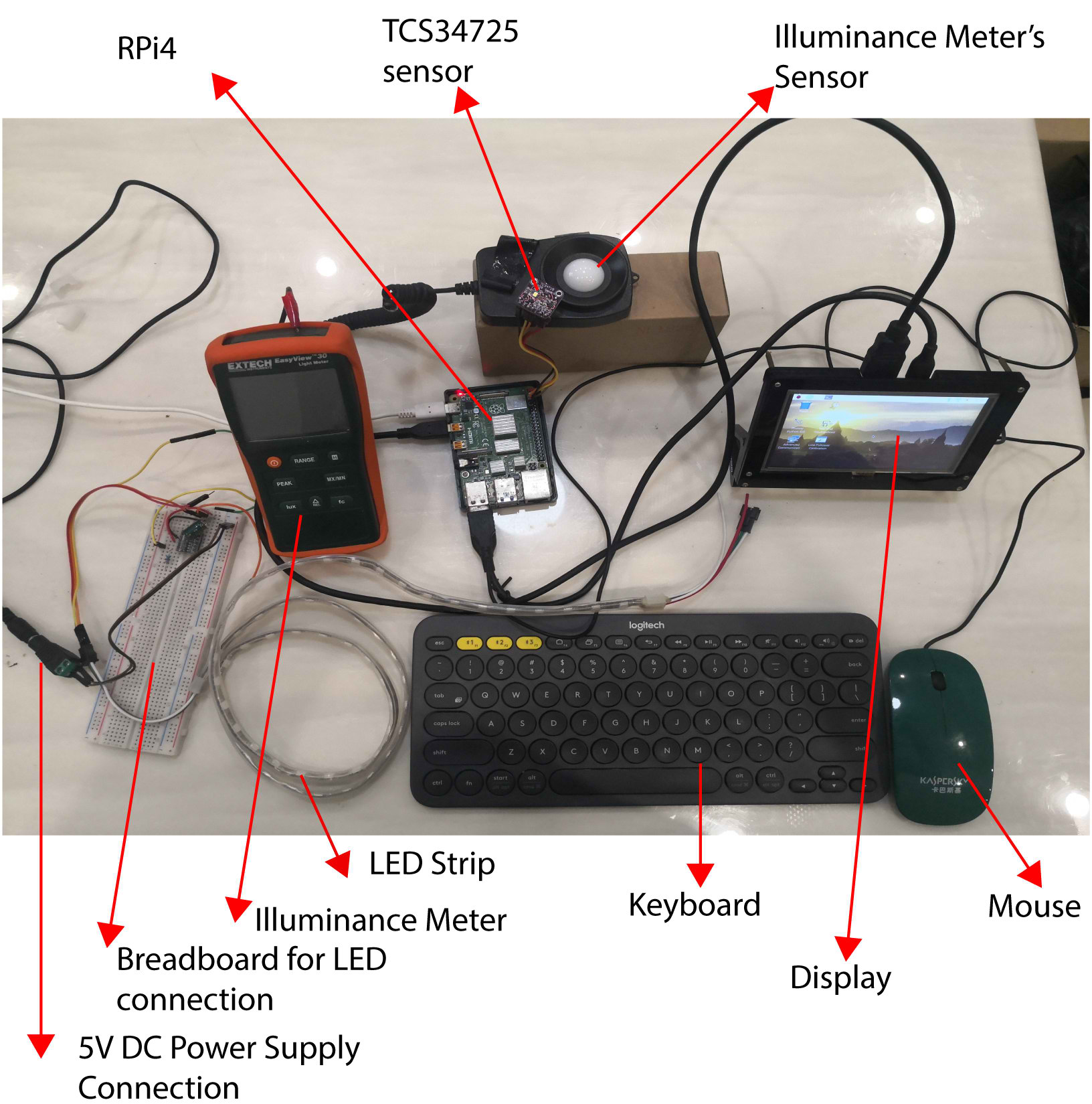
Fig. 19. Entire prototype set-up and accessories.

3.2. Fuzzy logic controller analysis

Figure 20 depicts the controller’s output performance when running a single loop. The target colour swatch was set randomly at 4954 K. The room colour swatch parameters correlate with the measurements from the RGB colour sensor. The colour has been converted to RGB display form. The command from the FLC system controller is named ’corrFLC,’ i.e., the colour that the controller commands the LED lighting to display.

Figure 20

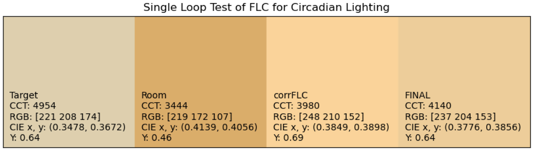
Fig. 20. Single loop test of a lighting controller.

The FLC aims to match “Target” and “Final” swatches through multiple loops. Due to colour mixing, the room will eventually appear as the colour swatch designated “Final.” However, after running multiple loops through the control system’s error correction technique, the colour properties of the “Final” swatch would converge and match the “Target” requirements. The “Final” swatch is a spectrum-wise data addition between “Room” and “corrFLC” spectrums which resulted as such. Conversion from CIE xyY parameters to RGB also resulted in out-of-gamut values for certain cases, which required clipping of max and min values to between 0 and 1.

A trial-and-error method was used to determine the number of fuzzy sets required for each input. As illustrated in Fig. 21, an initial assessment with three errors and a change in errors resulted in an underperforming control system. The universe of discourse of input variables was divided equally, as in Table 7. Abbreviations: N – Negative, ZO – Zero, P – Positive, S – Small, M- Medium, and L – Large apply. The values in the table field represent the consequents of each rule.

Figure 21

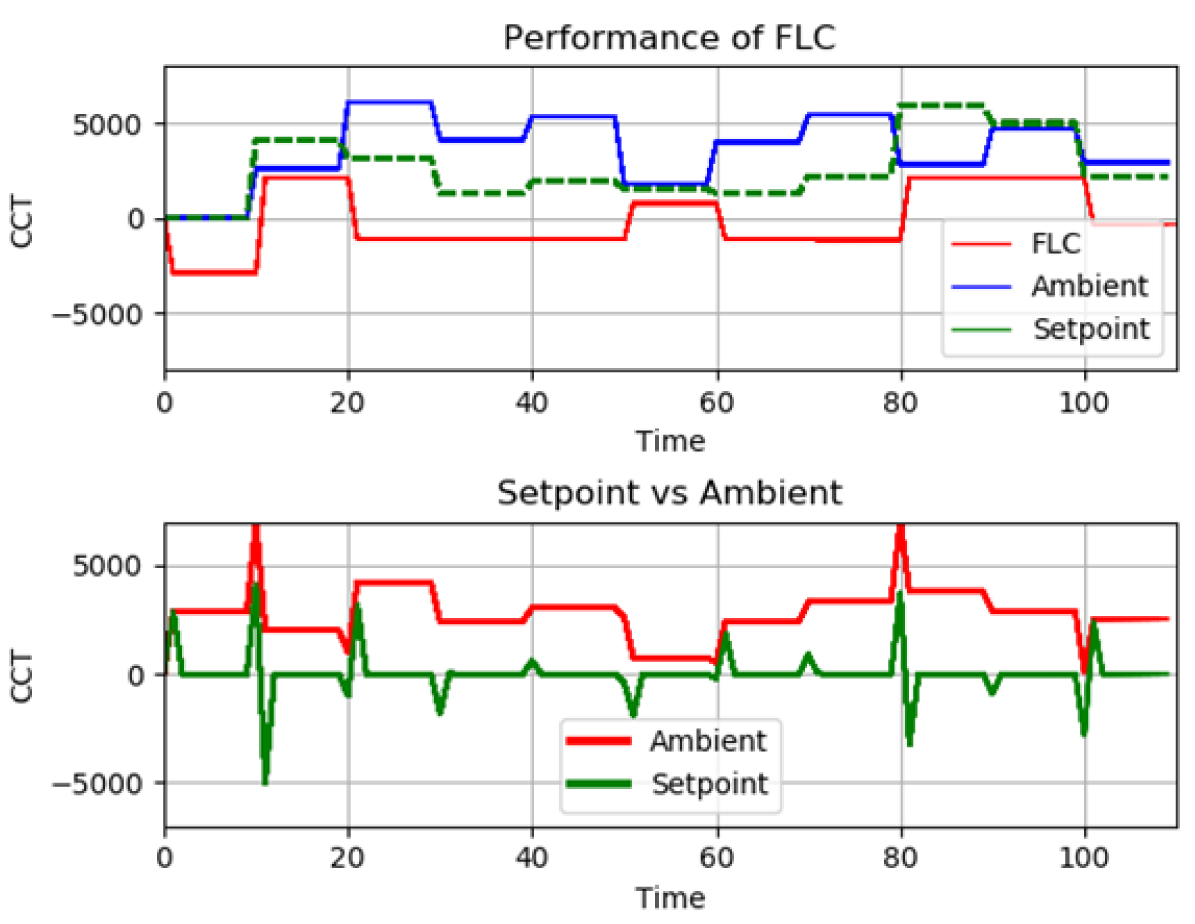
Fig. 21. FLC compensation response (3x3 inputs vs 3 fuzzy output sets).

Table 7

Table 7. Fuzzy input variables assigned three fuzzy sets (N, Z, P).

For a 3×3 rule matrix, the red line on the top plot in Fig. 21 depicts the FLC’s output compared to ambient (room) and setpoint settings. The FLC compensation output (red line) follows the setpoint and compensates for ambient inaccuracies, resulting in acceptable performance. However, the tracking performance can further be improved. For example, between the relative time interval of 20th to 50th iteration, the red line (FLC) seems static for slight changes in setpoint and ambient data. In actual performance, the output from the controller is minute.

Using a 7×5 sets of fuzzy inputs and outputs, as shown in Table 8, the FLC’s performance is further optimised and improved. The decision to use 7×5 sets is based on trials and experiences. Figure 22 depicts the fuzzification sets for the inputs. The shape of membership functions is similar for error, Δe and output Δu.

Table 8

Table 8. Fuzzy input variables assigned 7×5 fuzzy sets (NL, NM, NS, ZO, PS, PM, PL).

Figure 22

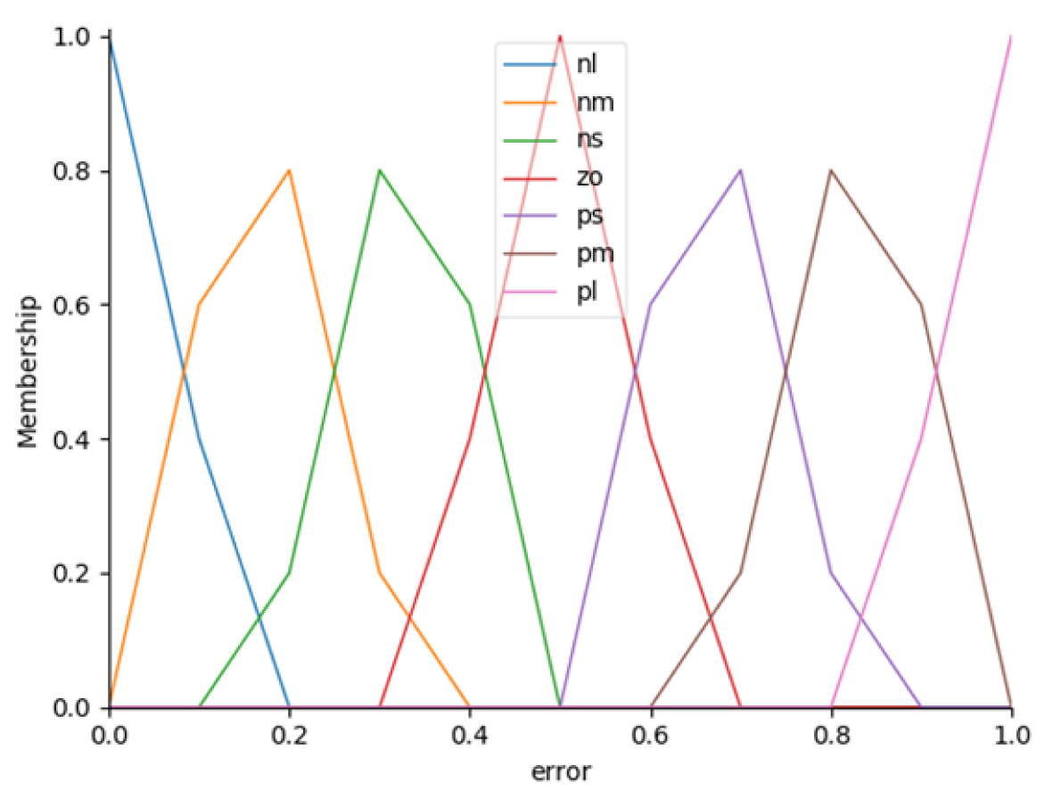
Fig. 22. Fuzzification of input to 7 fuzzy sets.

The FLC’s reaction has improved in Fig. 23, where the red line tracks to correct for changes in setpoint and ambient measurements like Fig. 21. However, minor changes and deviations are significantly considered. For example, the red line (FLC) tracks the shift in inputs from the relative time of 50th to 70th iterations.

Figure 23

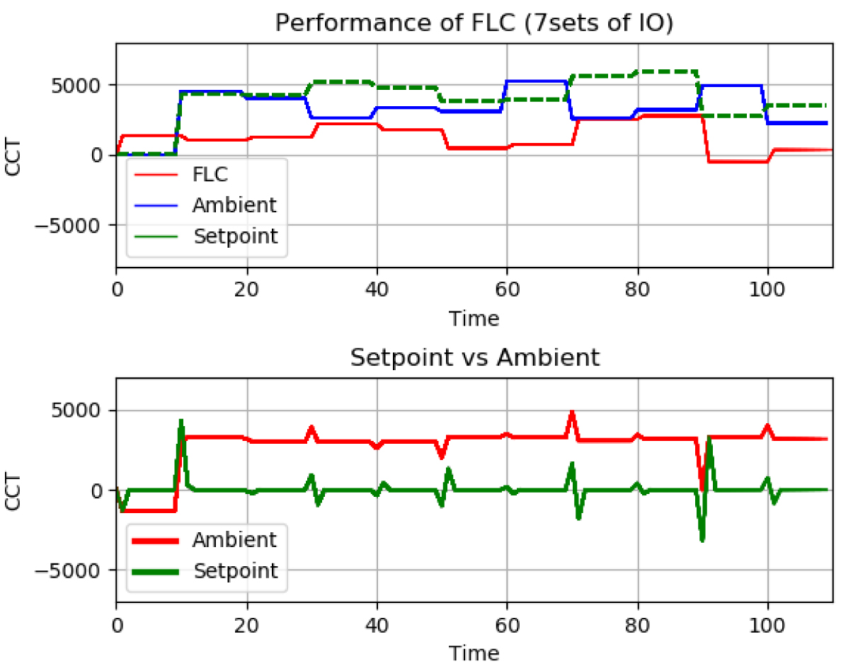
Fig. 23. FLC compensation response (7×5 inputs + 7 output fuzzy sets).

Figure 24 shows the performance of the FLC when simulated on continuous multiple open loops. Throughout the simulation run, the “final” CCT tracks the "target" or desired CCT successfully with a slight error whenever target CCT exceeds the room’s CCT. The error is due to the conversion process of SPD to CCT using McCamy’s formula and RGB conversions, which are nonlinear. In fact, McCamy’s formula is not suitable for CCT magnitudes lesser than 2000 K, as will be discussed in Section 4.0. In addition, Fig. 24 only highlights simulation results instead of actual readings. There will be stochastic noises introduced into the system for actual application, which would deviate from theoretical simulation results causing overshoots and transients. In control systems, overshoot is defined as the phenomenon exceeding of the control response signal compared to the desired value. Transients on the other hand, are like overshoots, however they have a repetitive characteristic that imparts on the response signal and may be positive or negative with respect to the desired value. To solve the deviation issue, a closed-loop FLC controller system is utilised. The FLC will determine the compensation to achieve near-target values, and the closed-loop system corrects the minor deviations. Nevertheless, the FLC is robust to consider the large deviations.

Figure 24

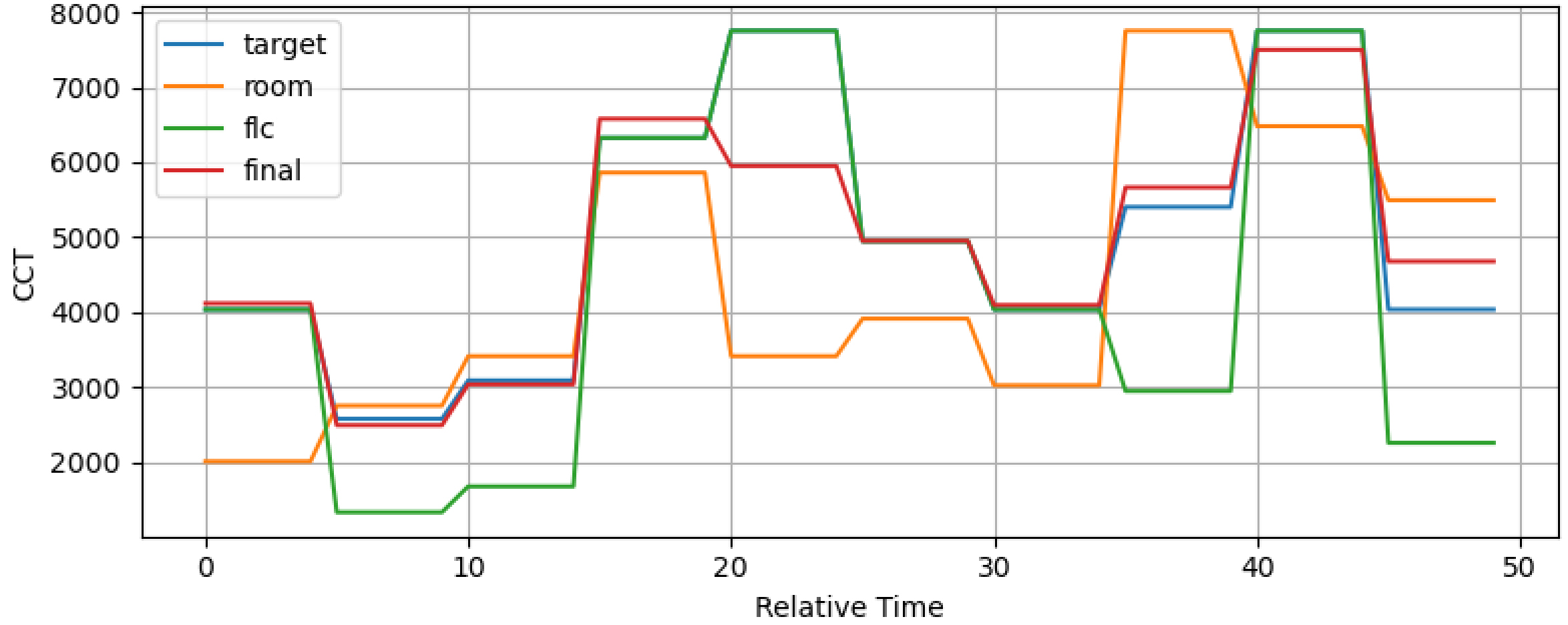
Fig. 24. Performance of FLC in simulated continuous open loops.

The same fuzzy rule matrix is reused in a closed loop with the proportional gain set at unity for a continuous loop with error correction. Figure 25 shows the results, but the response is acceptable as steady state is reached at about 4th iteration (relative time). Table 9 tabulates the attributes of the closed-loop response. The performance may be improved to achieve a faster steady-state by integrating a PID controller in the hybrid closed-loop system. PID integration is beyond the scope of this research and is an idea for future works. Figure 26 shows a test run of several different desired values. The closed-loop FLC system was robust enough to track the desired value.

Figure 25

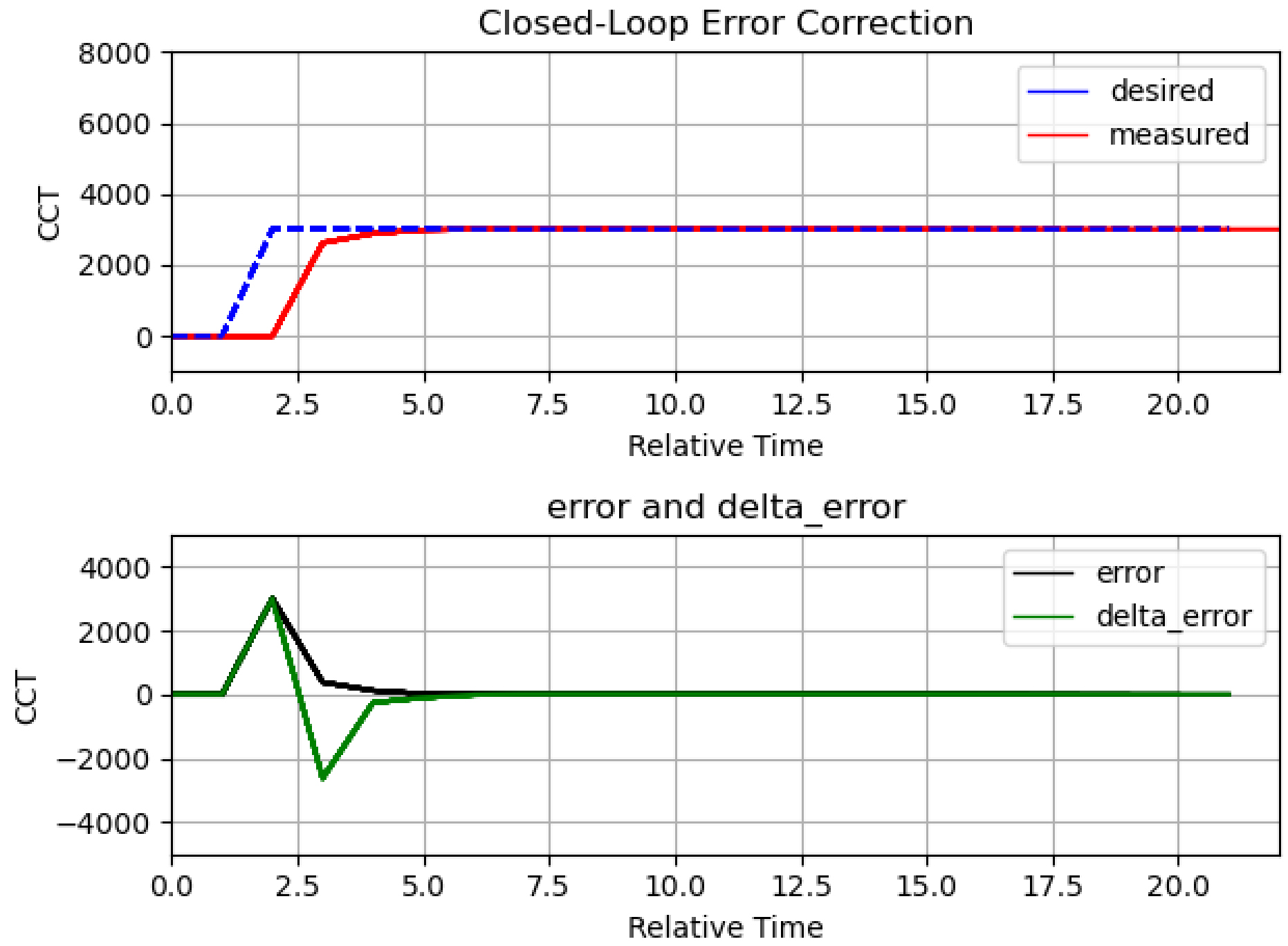
Fig. 25. Error Correction in Closed-Loop with single target.

Table 9

Table 9. Closed-loop response attributes.

Figure 26

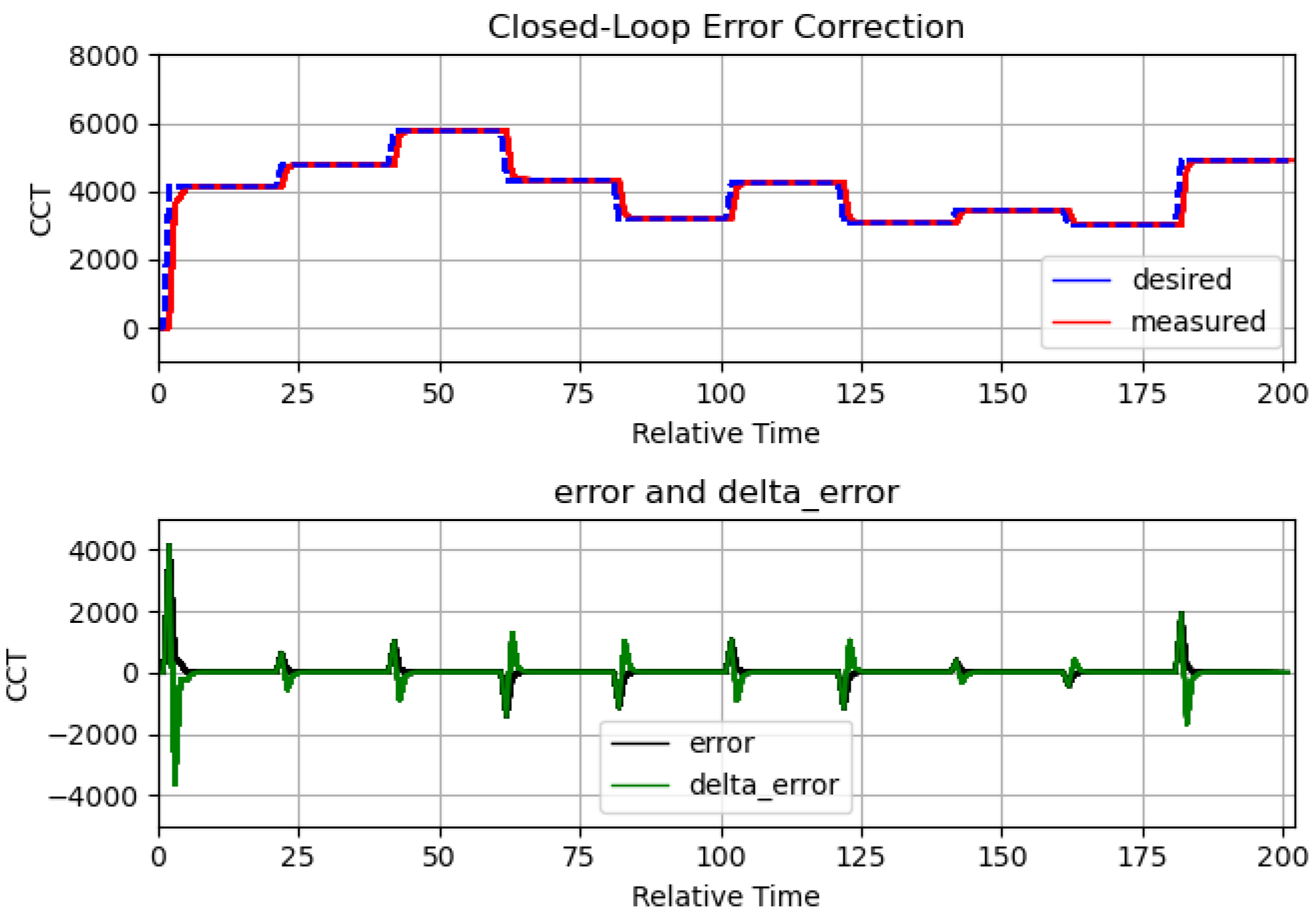
Fig. 26. Error Correction in Closed-Loop with multiple targets.

Signals were transferred from the minicomputer to the LED strips once the LED lighting prototype was built to evaluate and simulate distinct colour renderings. Table 10 below tabulates some of the CCT to RGB values calculated using earlier methods. The Duv error is within ±0.003, signifying the colours are within the white area.

Table 10

Table 10. CCT and RGB values calculated from minicomputer.

3.3. LED lighting output

Figure 27 shows a short LED strip that was evaluated and can render warm (first picture) to cool (second picture) colours, as well as combinations of warm and cool colours (third picture). The three primary colours, Red, Green, and Blue, are rendered in the far-right image.

Figure 27

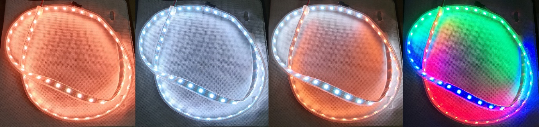
Fig. 27. LED lighting strip producing variable tones of colours.

A detailed test scenario for the lighting control system with data is summarised in Table 11 below. The appearance of the LED strip was evaluated as per the findings in Table 11 that is to output 4148 K, as shown in Fig. 28. Figure 29 shows the Illuminant D spectrum generated throughout the fuzzy logic compensation process corresponding to Table 11, where the "Final" spectrum closely follows the "Target" spectrum.

Table 11

Table 11. Sample Calculation and Data Processing of Smart Lighting.

Figure 28

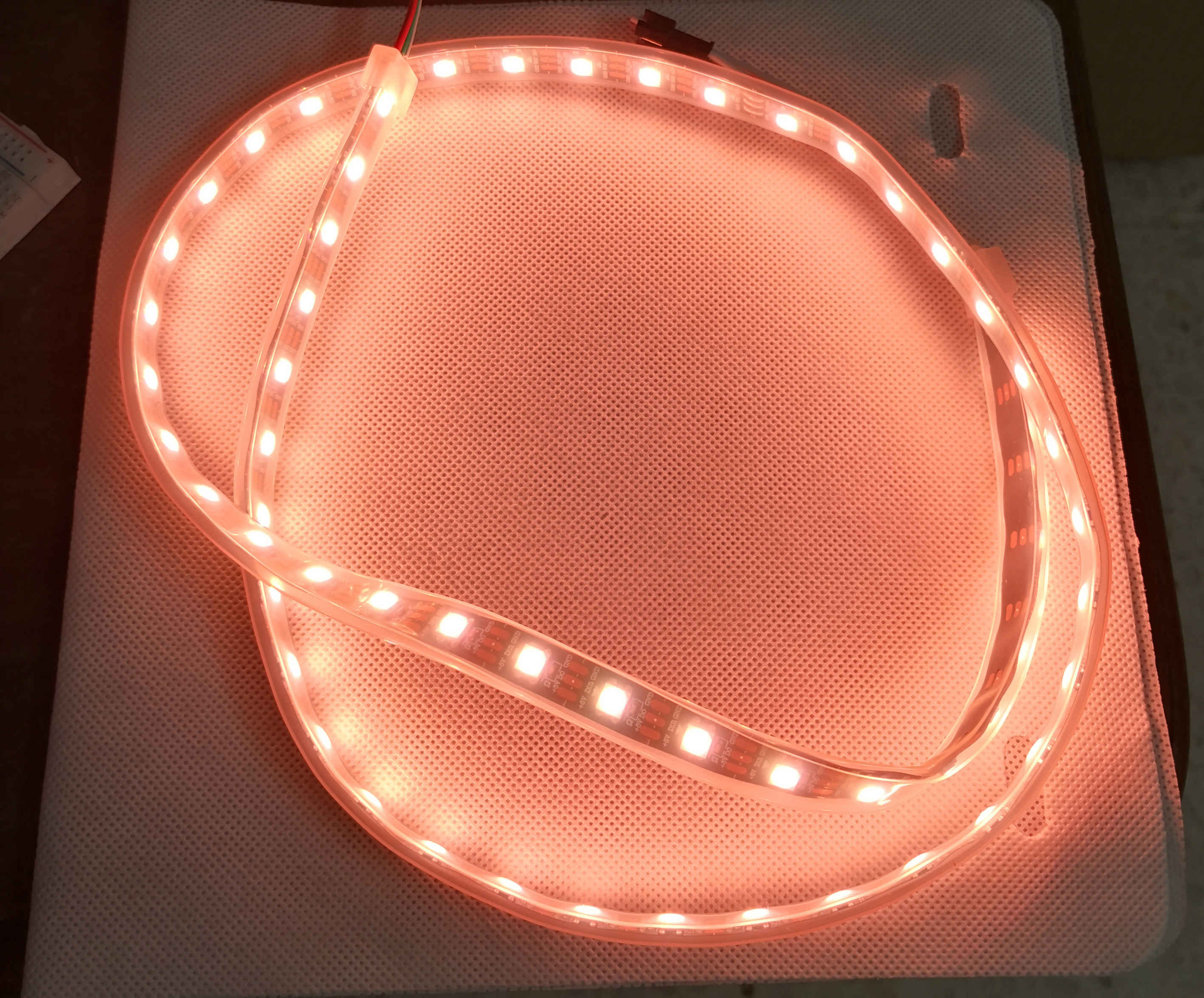
Fig. 28. LED lighting strip producing 4148 K CCT.

Figure 29

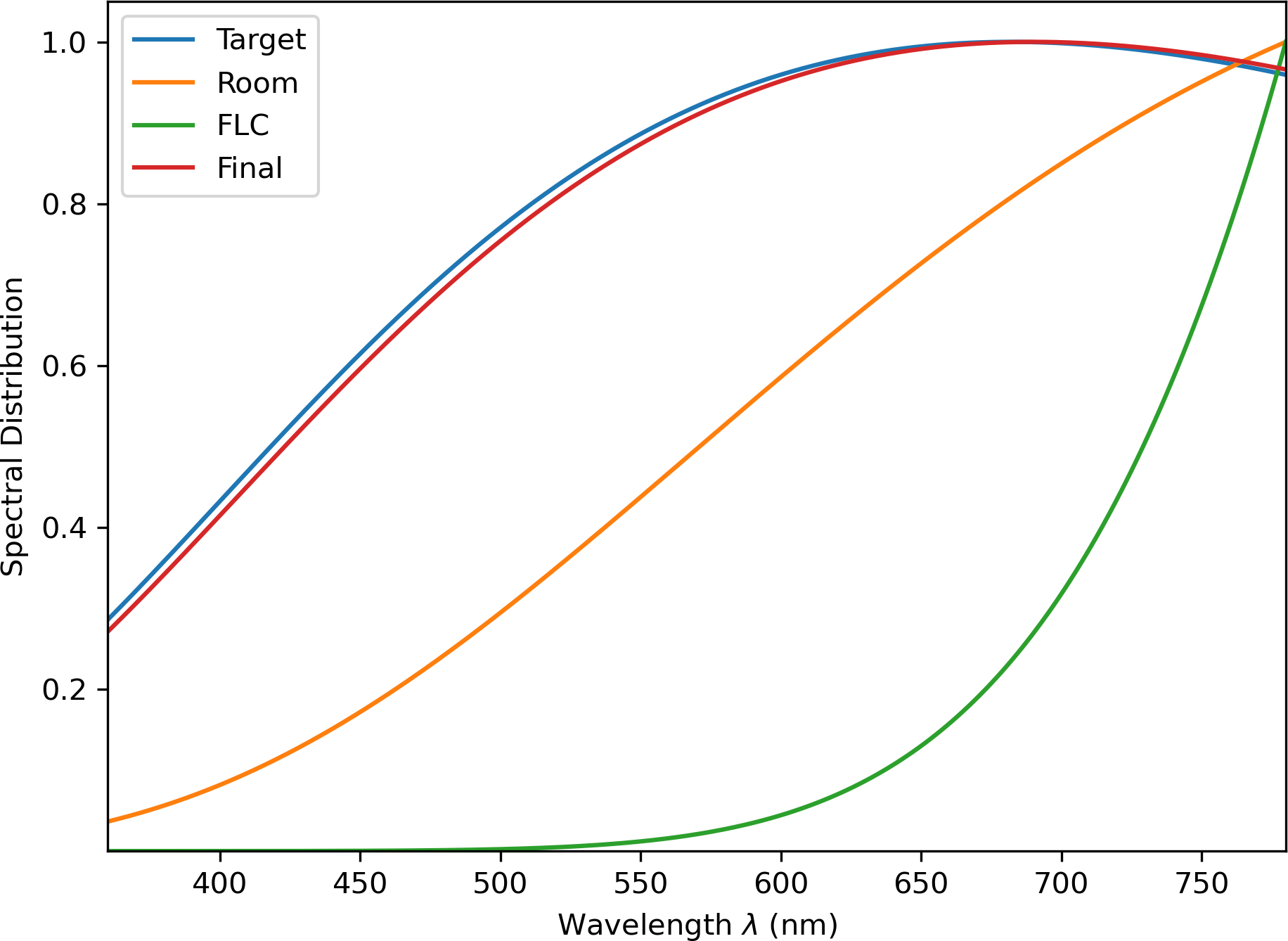
Fig. 29. SPD for various lighting parameters in FLC compensation process.

4. Discussion

FLC application to lighting spectrums manipulation is deemed appropriate due to the characteristics of lighting itself, where fuzziness exists. As various unwanted disturbance lighting is introduced, the FLC system can tackle the concern as modelling and derivation of the process’s transfer function is not required. To have a much better response, a hybrid integration between PID and FLC system application may be more robust for the control system output accuracy. Also, this may be a consideration for future works.

In the initial research and project planning phase, it was planned to use the idea of using external sensors instead of the Table 5 fixed time-CCT database. However due to the minicomputer’s limitation of only having single serial clock pin (SCL) and serial data pin (SDA), only one sensor could be used. Thus, the outdoor CCT characteristics was arbitrarily defined to have a full range of CCTs spread across 24 hours. Therefore, adding another sensor (or more) through the I2C (serial) communication interface is impossible. One way of overcoming to, to cascade several RPI4 (minicomputer) attached to a single sensor, and each linked to a central RPi4. Such approach is deemed costly and tedious but do-able through additional RPi4 board tweaking and considered for future works.

On the the other hand, the generated SPD through Planckian equation resembles CIE Illuminant D spectrums. Though there is a approximate modelling equation to produce the SPD from CIE xy chromaticity coordinates, this research utilized the Planckian equation, as there is a future plan to integrate several spectrometric sensors which could measure full spectral irradiance of the outdoor and lighting space [17,29,40]. When, this is made possible, the FLC system can start compensating each wavelength-intensity individually instead on averaged single parameters such as CCT. Current design maximised cost efficiency and focused on FLC compensation. Thus, a true SPD replication can be engineered with spectrometric sensors. The spectrometric sensors to measure outdoor SPD can be placed at building facades or roof-mounted. This plan becomes an idea for future work.

Although the error correction through a closed-loop system shows clean results in the simulation, the validity of McCamy’s formula becomes a concern in practical applications. The usage of McCamy’s formulas as in Eq. 15 only applies to a range of, at most, 1621 K to 34530 K. As error decreases in subsequent iterations, the usage of the formula is not accurate anymore. However, out of range RGB values are clipped to be within the sRGB gamut, which means the extreme colour is fixed to be either white or black. One alternative is to use the Robertson method [44] or Li method [47], which needs transformation to another colour space environment, namely CIE 1960 UCS colour space, but involves many computations. Thus, these limitations can be a consideration for future works.

An example of this design may be applied at hospital wards. Fig 30 shows a diagram of hospital open ward configured to apply the proposed system. Hospital wards have patients where illness recovery time is essential. Studies have shown that circadian lighting introduction to wards improved patient’s rehabilitation time [9,48]. In fact, circadian lighting application has also reduced medical errors and dispensing errors at wards and pharmacies [49–51].

In Fig. 30, the open ward has been populated with LED lighting and sensors. The wards can be zoned, and each zone may be applied distinct CCT. For example, Grid C1 has warm colours whereas grid F5 has cool colours. The control unit (RPi4) can distinctly control each pixel of the LED lighting strip to render colours based on occupants' need.

Figure 30

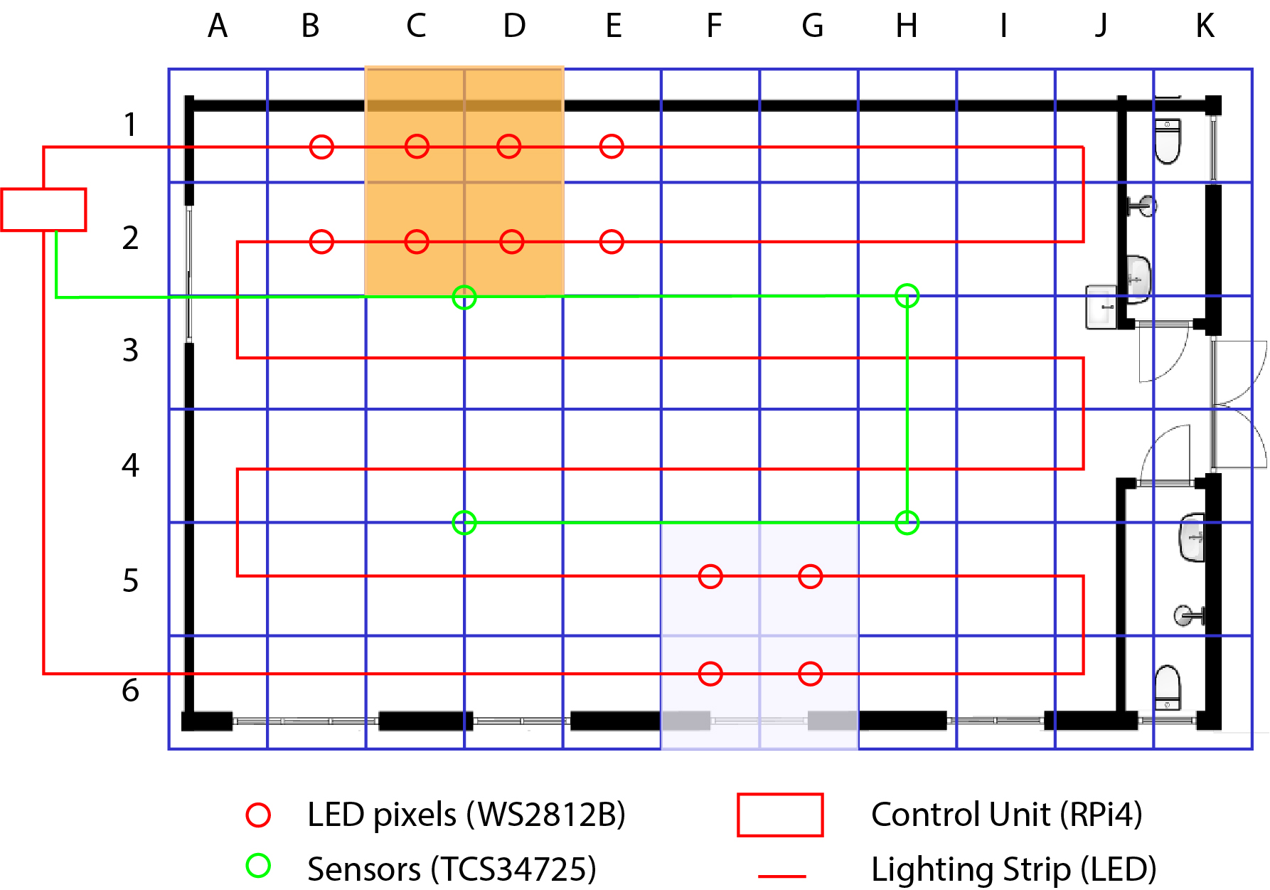
Fig. 30. Application strategy for the lighting FLC system.

5. Conclusions

Circadian lighting is a lighting that follows the natural lighting characteristics which affects human beings sleep and wake patterns. Combining artificial lighting to match natural outdoor lighting characteristics through CCT variations enhances occupant comfort and well-being (NIF effect). An FLC was employed to regulate lighting with specific characteristics in terms of the colour content (SPD spectrum). FLC is cost-efficient, easily applied or developed and versatile. It requires minor tuning when ported from one system to another. In a closed-loop control system, the FLC was programmed to replicate natural lighting characteristics corresponding to the time mark in a day. A database of time-CCT was devised to simulate the system. The execution of circadian lighting replication consisted of transforming the lighting detected into CIE XYZ tristimulus values which could later be converted to RGB format, that LED luminaires can interpret and render. Deviation of CCT from white light region was measured to be at less than 1%, whereas response traits of the control system were excellent. Simulation results showed that the compensated CCT adjusted the final room CCT to match to desired CCT. The methodology can be adapted and expanded to large scale-built environment applications with spectrometric sensors.

Acknowledgement

The authors would like to thank the Ministry of Health, Malaysia, and University Sains Malaysia to make available research scholarship, data, tools, and support for publishing this article.

Contributions

SR Perumal suggested the concept, evaluated it, gathered data, and oversaw the article’s writing. F Baharum supervised the experiment and provided data analysis, debate, and assistance in cross-checking perspectives to develop this article.

Declaration of competing interest

This paper did not disclose any private, personal, and confidential data of anyone or organisations. The images are self-developed by the authors or from the stated sources (if any) for academic purposes.

References

P. Boyce, Human factors in lighting., 2nd ed., Taylor & Francis, 2003. https://doi.org/10.1201/9780203426340
P.R. Mills, S.C. Tomkins, L.J.M. Schlangen, The effect of high correlated colour temperature office lighting on employee wellbeing and work performance, J. Circadian Rhythms. 5 (2007) 2. https://doi.org/10.1186/1740-3391-5-2
M. Rossi, Circadian Lighting Design in the LED Era, Springer International Publishing, Cham, 2019. https://doi.org/10.1007/978-3-030-11087-1
X. Xuan, Study of indoor environmental quality and occupant overall comfort and productivity in LEED- and non-LEED-certified healthcare settings, Indoor Built Environ. 27 (2018) 544-560. https://doi.org/10.1177/1420326X16684007
Y. Hua, A. Oswald, X. Yang, Effectiveness of daylighting design and occupant visual satisfaction in a LEED Gold laboratory building, Build. Environ. 46 (2011) 54-64. https://doi.org/10.1016/j.buildenv.2010.06.016
Malaysia Carbon Reduction & Environmental Sustainability Tool V2, Kuala Lumpur, Malaysia, 2020.
Y. Zhu, M. Yang, Y. Yao, X. Xiong, X. Li, G. Zhou, N. Ma, Effects of Illuminance and Correlated Color Temperature on Daytime Cognitive Performance, Subjective Mood, and Alertness in Healthy Adults, Environ. Behav. 51 (2019) 199-230. https://doi.org/10.1177/0013916517738077
P. Boyce, Review: The Impact of Light in Buildings on Human Health, Indoor Built Environ. 19 (2010) 8-20. https://doi.org/10.1177/1420326X09358028
N.P. Hoyle, E. Seinkmane, M. Putker, K.A. Feeney, T.P. Krogager, J.E. Chesham, L.K. Bray, J.M. Thomas, K. Dunn, J. Blaikley, J.S. O'Neill, Circadian actin dynamics drive rhythmic fibroblast mobilization during wound healing, Sci. Transl. Med. 9 (2017) eaal2774. https://doi.org/10.1126/scitranslmed.aal2774
M.J. Patyra, D.M. Mlynek, Fuzzy Logic: Implementation and Applications, Vieweg+Teubner Verlag, Wiesbaden, 2012. https://doi.org/10.1007/978-3-322-88955-3
D.J. Norris, Beginning Artificial Intelligence with the Raspberry Pi, Apress, Berkeley, CA, 2017. https://doi.org/10.1007/978-1-4842-2743-5
A.Q. Ansari, The basics of fuzzy logic: A tutorial review, Comput. Educ. Educ. GROUP-. 88 (1998) 5-8.
P.J. King, E.H. Mamdani, The application of fuzzy control systems to industrial processes, Automatica. 13 (1977) 235-242. https://doi.org/10.1016/0005-1098(77)90050-4
P. Singhala, D. Shah, B. Patel, Temperature Control using Fuzzy Logic, Int. J. Instrum. Control Syst. (2014).
M. Rasemabuzeid, N.E. Shtawa, Comparative Speed Control Study Using PID and fuzzy Logic Controller, Int. J. Comput. Sci. Electron. Eng. 2 (2014).
I. Chew, V. Kalavally, N.W. Oo, J. Parkkinen, Design of an energy-saving controller for an intelligent LED lighting system, Energy Build. 120 (2016) 1-9. https://doi.org/10.1016/j.enbuild.2016.03.041
I. Chew, V. Kalavally, C.P. Tan, J. Parkkinen, A spectrally tunable smart LED lighting system with closed-loop control, IEEE Sens. J. 16 (2016) 4452-4459. https://doi.org/10.1109/JSEN.2016.2542265
G. Cimini, A. Freddi, G. Ippoliti, A. Monteriù, M. Pirro, A Smart Lighting System for Visual Comfort and Energy Savings in Industrial and Domestic Use, Electr. Power Components Syst. 43 (2015) 1696-1706. https://doi.org/10.1080/15325008.2015.1057777
J. Warner, J. Sexauer, scikit-fuzzy, twmeggs, alexsavio, A. Unnikrishnan, G. Castelão, F.A. Pontes, T. Uelwer, pd2f, laurazh, F. Batista, alexbuy, W. Van den Broeck, W. Song, T.G. Badger, R.A.M. Pérez, J.F. Power, H. Mishra, G.O. Trullols, A. Hörteborn, 99991, JDWarner/scikit-fuzzy: Scikit-Fuzzy version 0.4.2, (2019). https://doi.org/10.5281/zenodo.3541386
Y.A. Almatheel, A. Abdelrahman, Speed control of {DC} motor using Fuzzy Logic Controller, in: 2017 Int. Conf. Commun. Control. Comput. Electron. Eng., IEEE, 2017. https://doi.org/10.1109/ICCCCEE.2017.7867673
J. Liu, W. Zhang, X. Chu, Y. Liu, Fuzzy Logic Controller for Energy Savings in a Smart LED Lighting System Considering Lighting Comfort and Daylight, Energy Build. 127 (2016) 95-104. https://doi.org/10.1016/j.enbuild.2016.05.066
H.-T. Chen, S.-C. Tan, S.Y. Hui, Nonlinear dimming and correlated color temperature control of bicolor white LED systems, IEEE Trans. Power Electron. 30 (2014) 6934-6947. https://doi.org/10.1109/TPEL.2014.2384199
A.T.L. Lee, H. Chen, S.-C. Tan, S.Y. Hui, Precise dimming and color control of LED systems based on color mixing, IEEE Trans. Power Electron. 31 (2015) 65-80. https://doi.org/10.1109/TPEL.2015.2448641
S. Buso, G. Spiazzi, White light solid state lamp with luminance and color temperature control, in: XI Brazilian Power Electron. Conf., 2011: pp. 837-843. https://doi.org/10.1109/COBEP.2011.6085167
H. Kim, J. Liu, H.-S. Jin, H.-J. Kim, An LED color control system with independently changeable illuminance, in: INTELEC 2009-31st Int. Telecommun. Energy Conf., 2009: pp. 1-5. https://doi.org/10.1109/INTLEC.2009.5351875
Y. Gao, H. Wu, J. Dong, G.Q. Zhang, Constrained optimization of multi-color LED light sources for color temperature control, in: 2015 12th China Int. Forum Solid State Light., 2015: pp. 102-105. https://doi.org/10.1109/SSLCHINA.2015.7360699
S. Muthu, F.J. Schuurmans, M.D. Pashley, Red, green, and blue LED based white light generation: issues and control, in: Conf. Rec. 2002 IEEE Ind. Appl. Conf. 37th IAS Annu. Meet. (Cat. No. 02CH37344), 2002: pp. 327-333. https://doi.org/10.1109/IAS.2002.1044108
J. Schanda, Colorimetry. understanding the CIE system., John Wiley & Sons, 2007. https://doi.org/10.1002/9780470175637
I. Fryc, S.W. Brown, G.P. Eppeldauer, Y. Ohno, LED-based spectrally tunable source for radiometric, photometric, and colorimetric applications, Opt. Eng. 44 (2005) 111309. https://doi.org/10.1117/1.2127952
RS-Components, Datasheet Raspberry Pi Model B, Raspberrypi.Org. (2019) 1.
TAOS, Datasheet - TCS34725 - Color Light-to-Digital Converter with IR Filter, (2012) 1-26. www.taosinc.com.
S.R. Perumal, and Faizal Baharum, Measurement, Simulation, and Quantification of Lighting-Space Flicker Risk Levels Using Low-Cost {TCS}34725 Colour Sensor and {IEEE} 1789-2015 Standard, J. Daylighting. 8 (2021) 239-254. https://doi.org/10.15627/jd.2021.19
P. Boyce, P. Raynham, The SLL Lighting Handbook, The Society of Light and Lighting, London, 2009.
A.E.F. Taylor, others, Illumination fundamentals, Light. Res. Center, Rensselaer Polytech. Inst. 22 (2000).
International Telecommunication Union, Parameter values for the HDTV standards for production and international programme exchange BT Series Broadcasting service, Recomm. ITU-R BT.709-5. 5 (2002) 1-32. http://www.itu.int/dms_pubrec/itu-r/rec/bt/R-REC-BT.709-5-200204-I!!PDF-E.pdf.
M. Bertalmio, Vision models for high dynamic range and wide colour gamut imaging: techniques and applications, Academic Press, 2019. https://doi.org/10.1016/B978-0-12-813894-6.00015-6
C. Poynton, Gamma FAQ--frequently asked questions about gamma, (2002).
C.S. McCamy, Correlated color temperature as an explicit function of chromaticity coordinates, Color Res. Appl. 17 (1992) 142-144. https://doi.org/10.1002/col.5080170211
Y. Ohno, Practical use and calculation of CCT and Duv, Leukos. 10 (2014) 47-55. https://doi.org/10.1080/15502724.2014.839020
I. Fryc, S.W. Brown, Y. Ohno, Spectral matching with an LED-based spectrally tunable light source, in: Fifth Int. Conf. Solid State Light., 2005: p. 59411I. https://doi.org/10.1117/12.614952
T. Mansencal, M. Mauderer, M. Parsons, N. Shaw, K. Wheatley, S. Cooper, J.D. Vandenberg, L. Canavan, K. Crowson, O. Lev, others, Colour 0.3. 16, Zenodo, Jan. 25 (2020).
P. Virtanen, R. Gommers, T.E. Oliphant, M. Haberland, T. Reddy, D. Cournapeau, E. Burovski, P. Peterson, W. Weckesser, J. Bright, S.J. van der Walt, M. Brett, J. Wilson, K.J. Millman, N. Mayorov, A.R.J. Nelson, E. Jones, R. Kern, E. Larson, C.J. Carey, \.Ilhan Polat, Y. Feng, E.W. Moore, J. VanderPlas, D. Laxalde, J. Perktold, R. Cimrman, I. Henriksen, E.A. Quintero, C.R. Harris, A.M. Archibald, A.H. Ribeiro, F. Pedregosa, P. van Mulbregt, SciPy 1.0 Contributors, {SciPy} 1.0: Fundamental Algorithms for Scientific Computing in Python, Nat. Methods. 17 (2020) 261-272. https://doi.org/10.1038/s41592-019-0686-2
World-Semi, WS2812B V5 5050 LED Datasheet, Worldsemi. (2019).
A.R. Robertson, Computation of Correlated Color Temperature and Distribution Temperature, J. Opt. Soc. Am. 58 (1968) 1528. https://doi.org/10.1364/JOSA.58.001528
Osram Sylvania, Light can be white, white, white or white. white, (1995).
EN 12464-1: 2011 Light and Lighting-Lighting of Work Places-Part 1: Interior Work Places, CEN Brussels, Belgium, 2011.
C. Li, G. Cui, M. Melgosa, X. Ruan, Y. Zhang, L. Ma, K. Xiao, M.R. Luo, Accurate method for computing correlated color temperature, Opt. Express. 24 (2016) 14066. https://doi.org/10.1364/OE.24.014066
J.-H. Choi, L.O. Beltran, H.-S. Kim, Impacts of indoor daylight environments on patient average length of stay (ALOS) in a healthcare facility, Build. Environ. 50 (2012) 65-75. https://doi.org/10.1016/j.buildenv.2011.10.010
L.J. McCunn, J. Wright, Hospital employees' perceptions of circadian lighting: a pharmacy department case study, J. Facil. Manag. 17 (2019) 422-437. https://doi.org/10.1108/JFM-04-2019-0016
T.L. Buchanan, K.N. Barker, J.T. Gibson, B.C. Jiang, R.E. Pearson, Illumination and errors in dispensing., Am. J. Hosp. Pharm. 48 (1991) 2137-45. https://doi.org/10.1093/ajhp/48.10.2137
M. Engwall, I. Fridh, L. Johansson, I. Bergbom, B. Lindahl, Lighting, sleep and circadian rhythm: An intervention study in the intensive care unit, Intensive Crit. Care Nurs. 31 (2015) 325-335. https://doi.org/10.1016/j.iccn.2015.07.001

Get PDF (12.4 MB)

SHARE ON